The Consequences of Fixed Time Performance Measurement*

John L. Gustafson

Table of Contents

Abstract

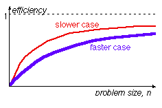
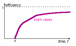
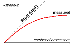
In measuring performance of parallel computers, the usual method is to choose a problem and test execution time as the processor count is varied. This model underlies definitions of "speedup," "efficiency," and arguments against parallel processing such as Ware's formulation of Amdahl's law. Fixed time models use problem size as the figure of merit. Analysis and experiments based on fixed time instead of fixed size have yielded surprising consequences: The fixed time method does not reward slower processors with higher speedup; it predicts a new limit to speedup, more optimistic than Amdahl's; it shows efficiency independent of processor speed and ensemble size; it sometimes gives non-spurious superlinear speedup; it provides a practical means (SLALOM) of comparing computers of widely varying speeds without distortion.

1. Introduction

The main reason we use computers is speed. True, they often produce work of higher quality and reliability than other means of doing a task, but these are really just forms of speed. With enough time, pencil-and-paper calculations can match the quality and reliability of a computer. It is the speed of computers that lets us do things we otherwise would not try.

The reason we use parallel computers instead of serial computers is also for speed. This seems so obvious that we seldom belabor the point. Yet, we base everything we do in parallel computing on this motive. The problem is that our usual definition of "speed" is not on very firm ground. Most papers skirt the issue of absolute speed and instead report "speedup," defining speedup strictly as time reduction.

The following cynical definition by Ambrose Bierce, from The Devil's Dictionary (1911), shows the absurdity of basing parallel performance on time reduction:

Bierce used this reasoning as humor almost a century ago. Now we call the flaw in the reasoning "Amdahl's law" and treat it as a serious obstacle to parallel performance. By scaling the problem to sixty post-holes, the absurdity disappears and the sixty men are sixty times as productive as a single man. My thesis is that parallel performance should be measured by the work done in fixed time, and not by time reduction for a fixed problem.

2. Myths of Performance Measurement

It seems clear that speed, for a computer, is work divided by time. But, what is "work"? The following common "myths" of speed and performance measurement illustrate difficulties involved in defining work:

2.1 Myth: The "work" is the operation count.

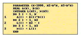
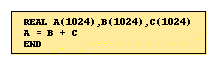
A Fortran example shows the fallacy of this idea:

Figure 1. FLOP-Count Counterexample

The only floating point operations are in the DO 1 loop, which has order N complexity. By current convention for measuring MFLOPS, the work in this problem is 103. However, the DO 2 loop has integer operations and is of order N2 complexity. Even the oldest digital computers would be misjudged by ignoring the relative cost of 106 integer operations, despite their much higher times for floating point operations. But, the DO 3 loop is the most troublesome since it has order N3 complexity and has no "operations" by common measures. Yet, memory operations are the most commonly-used instructions on computers.

The earliest computers were like humans in the respect that they took much longer to do arithmetic, especially multiplies, than to read operands or write results. The situation we now see, compute-intensive processors much faster at arithmetic than data motion, is not intuitive. In the early days of computing, gates (vacuum tubes) dominated both the system cost and the execution time; the wires connecting them were cheap by comparison. Current high-end computer costs and times are dominated by the connections, and the gates are cheap by comparison. Even recent numerical analysis texts base their complexity analysis on the economics of outdated arithmetic-bound machines.

2.2 Myth: The best serial algorithm defines the least work necessary.

In an example from Parkinson [22], elegantly expressed in Fortran 90, a serial processor might do more work than a parallel ensemble:

Figure 2. "Best Serial Algorithm" Counterexample

A serial processor can only do the operations with some type of loop that references each element in turn, as stored in linearly addressed memory. A data-parallel computer like a MasPar or Connection Machine does nothing so complicated. Each of 1024 processors only needs to compute three address references and one addition, with no loop management. One could argue that the elements had to be dispersed to the 1024 processors in the first place. But, this isn't true in the context of a larger application that contains the operation. Which defines the minimum work? The serial computer that must add, store the result, increment three memory pointers, test a loop counter, and branch? Or, a parallel computer that simply adds and stores the result? The example in Section 2.1 shows we cannot neglect simple overhead-type operations, no matter how trivial they may seem. A "proof" of the nonexistence of superlinear speedup by Faber, Lubeck, and White [10] relies implicitly on the assumption there is no savings from diminished loop overhead.

A similar counterexample occurs in tree-search problems. When a depth-first search is divided to run on a parallel computer, the resulting search is partly breadth-first. The breadth-first search sometimes does less work to find a particular goal. To reproduce the parallel search pattern on the serial computer involves extra serial work to change the entire "stem" in skipping from one part of the tree to another.

2.3. Myth: Peak MFLOPS ratings correlate well with application MFLOPS.

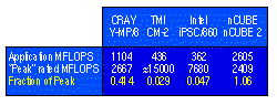
Counterexamples to this are rampant. To use a recent example that compares four very different computers, consider the following result from the "EP" Monte Carlo simulation taken from the NAS Parallel Benchmarks [4]:

Table 1a. Failure of Peak MFLOPS as Performance Predictor

Where is the pattern? All except the nCUBE use pipelined vector arithmetic. All except the CRAY are highly parallel. (This benchmark does almost no communication, so interprocessor speed ratings can be neglected.)

The nCUBE 2 exceeds "peak" speed because 64-bit floating point multiply-add operations determine the rated MFLOPS, but the benchmark involves roots, multiplies modulo 246, and logarithms counted as 12, 19, and 25 operations. The NAS weights are apparently based on CRAY Y-MP measurements. Since the nCUBE 2 does those things in less than 12, 19, and 25 times the time for a floating-point multiply or add, it exceeds its "peak speed."

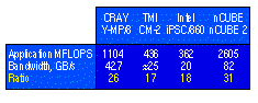
A partial resolution for this case appears if you use "peak memory bandwidth," the rate at which all the processors can use main memory (not cache) under ideal conditions:

Table 1b. Example of Memory Bandwidth as Performance Predictor

The bottom line is consistent enough to suggest that peak bandwidth instead of peak MFLOPS is a better simplistic predictor for this application. If peak MFLOPS correlated even weakly with observed rankings of computers, it would still be a practical tool for predicting performance. Alas, the failure of peak ratings even to rank computers correctly happens often in practice.

3. Background and Definitions

The previous section illustrated some of the current difficulties in assessing computer performance. The following section discusses historical attempts to analyze performance, especially parallel speed improvement. The definitions at the end of this section represent an attempt to provide a new theoretical basis for performance analysis that avoids some of the classical dilemmas.

3.1 A "Speedup" History

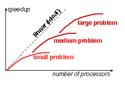
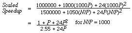
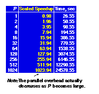
Twenty years ago, Ware [31] first summarized Amdahl's [2] arguments against multiprocessing as a speedup formula, popularly known as Amdahl's law. Amdahl's law shows a limit to performance enhancement. It was the only well-known parallel performance criterion until its underlying assumptions were questioned by Benner, Montry, and myself in our work at Sandia National Laboratory [14]. Based on experimental results with a 1024-processor system, we revised the assumptions of Amdahl and proposed the scaled speedup principle [13, [14]. Our argument was, and is, that parallel processing allows us to tackle previously out-of-reach problems. So, as problem size is increased with computing power, the serial component as defined by Amdahl and Ware cannot be regarded as constant.

Since then, researchers have sought a better understanding of parallel speedup. In 1989, Van-Catledge [30] and Zhou [34] studied the relation between Amdahl's law and scaled speedup. Eager et al. [9] studied speedup versus efficiency. Barton and Withers [5] developed a speedup model which considers the manufacturing cost of processors as a performance factor. In 1990, Karp and Flatt [18] suggested using the Amdahl-type serial fraction in an ad hoc sense. Worley showed the time constraints of scaled speedup [9]. Sun and Ni studied the relation between different speedup models [27], and Sun proposed a new metric to show aspects of the performance not easily seen from other metrics [29].

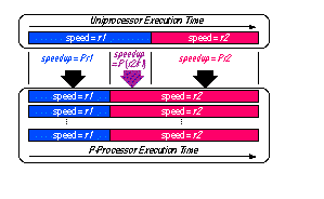
The definitions of "speedup" and "efficiency" are ingrained in the parallel processing literature. Speedup is the time on one processor divided by the time on P processors. Authors almost universally define speedup as sequential execution time over parallel execution time. The chosen sequential algorithm is the best sequential algorithm available, not the parallel algorithm run on one processor. (Sometimes the terms absolute speedup and relative speedup distinguish these approaches [29], with the latter meaning comparison with the parallel algorithm run on one processor.)

Efficiency is usually "speedup divided by P." For vector computers, efficiency often means operations per second divided by peak theoretical operations per second. Generally, speedup and efficiency depend on both N and P. Suppose C(N) represents the complexity of the best serial algorithm for a size N problem, and CP(N) is the complexity of the parallel algorithm run on P processors. Then

speedup (N, P) = C(N) / CP(N)(1)
efficiency (N, P) = speedup (N, P) / P(2)

Our scientific instincts tell us to control as many experimental variables as possible, and the most natural quantity to fix is N. It is becoming increasingly apparent that the restriction to constant N, though simple, is flawed and often misleading. In trying to find alternative definitions, we have found that time, not problem size, often serves better as a control variable when making scientific comparisons.

Forgetting for a moment the definition of speedup as "time reduction" that has become so ubiquitous in our industry, the English meaning would simply be "increase in speed." "Increase" is probably best translated mathematically as a ratio instead of a difference. We might define speedup as the speed on P processors divided by the speed on one processor. Only when work is constant does this simplify to the parallel processing definition of speedup [29].

3.2 Can We Define "Work"?

Although the goal of algorithm-independent, architecture-independent expressions for work is a laudable one, it is generally untenable.

The use of "speedup" as the ratio of times avoids the need for a rigorous definition of computational work, since the work in the numerators cancels out. To broaden the concept of speedup to variable problem sizes, we will need a practical definition of work. Operation count is an imperfect measure of computational work, since it does not standardize across computers. The counterexamples to Myths 1 and 2 illustrate this.

Even a simple word fetch from memory takes effort that varies with the computer. Is there error detection? Error correction? How large is the total memory containing the datum? Does the word size match the size of the data bus? Is the fetch word-aligned? In cache? Pipelined? Interleaved across memory banks?

Arithmetic is notoriously different from one computer to another. Specifying precision helps, but by no means creates a standard unit of "work." Computers with "64-bit arithmetic" might use from 47 to 56 bits for the mantissa, with the larger mantissas associated with more logic gates and precision. Not even use of the IEEE floating-point standard format promises fair comparison, since IEEE format does not ensure IEEE execution rules.

3.3 The "Standard Computer"

The most common approach is to pick a computer as representative, and define its execution time as the work. We see "VAX Units of Performance" and grand challenges that take work measured in "CRAY-centuries." As the counterexample to Myth 3 shows, picking a "standard computer" is hazardous business. In measuring the performance of homogeneous MIMD computers, one usually picks a single processor of the ensemble as the standard for comparison. Even then, system resources seldom scale perfectly with the number of processors.

Historically, people have assumed a "standard architecture computer," one that typifies the computers available at a given time. In the 1960's, this meant one could simply count floating-point multiplications in numerical algorithms and ignore everything else. By the 1970's, floating-point multiplies and adds had decreased to about the same cost. Both appeared in work measures based on "MFLOPS." The VAX-11/780 was commonly adopted as a standard for comparison. Since about 1980, scientific computers have taken longer to move data to and from main memory than to complete either type of floating point operation. Yet, our work measures have not caught up, and complexity analysis continues to concentrate on the quantity of arithmetic. The NAS Parallel Kernels [4] and Livermore Kernels [20] still use work measures based on weights for various types of floating-point arithmetic, where those weights follow from experience with the CRAY X-MP and CRAY Y-MP. To further complicate matters, the variety of machines commercially available is now far too great to hope for an application-independent performance ratio to a "standard architecture computer."

For now, we content ourselves with comparing single processors with collections of the same type in an ensemble. Even this restriction admits a simplification we call "The Flat Memory Approximation."

3.4 The Flat Memory Approximation

There are always limits on N for the coefficient fit. A common simplification in performance evaluation is to assume the complexity measure applies beyond the set of measurable sizes. When N becomes so large that the problem no longer fits in main memory, the computer must use secondary storage (either explicitly, or automatically via virtual memory). The coefficients in the functional form appear to increase for larger N, which is another way of saying that the functional form is too simple. It needs more terms to distinguish different memory reference types. Data caches have the opposite effect on the coefficient values. Figure 3 shows typical behavior for a computer with a data cache and virtual memory.

Figure 3. The Flat Memory Approximation

The program listing probably does not reveal the functional form of caching or virtual memory costs, making analysis very difficult. Even explicit use of secondary storage is hard to quantify, since it is usually mechanical and has random latency. So, many authors implicitly make the following assumption:

The Flat Memory Approximation: The empirical complexity for problems that fit
local memory serves for all problem sizes.

The Flat Memory Approximation is like the assumption that the Earth is flat. For many everyday activities, like estimating short distances, a planar view of the world simplifies life at little cost of accuracy. If we scale up the problem to distances of thousands of miles or down to a few inches, the flat Earth assumption gets us into trouble.

3.5 Serial Complexity

Assume we have picked a representative computer. We wish to know work as a function of N, the problem size. Examination of the control flow of a sequential algorithm on one processor of an ensemble yields an expression for the complexity C(N). All that matters is that the expression has the correct functional form. If a program contains even one loop construct containing a seemingly trivial operation of order N 5, then the expression must contain a term of that order. Knuth [19] provides dozens of examples of classical complexity analysis for serial algorithms.

The coefficients in the algebraic expression for C(N) can then be determined by experiment. Fitting timing curves to data avoids the need for operation weighting. For instance, there is disagreement over how to count a square root. Is it a single operation, as suggested by VAX-type architectures? Four operations, as defined for the Lawrence Livermore Kernels [20]? Twelve operations, as defined for the NAS Parallel Benchmarks [4]? It does not matter for purposes of performance evaluation. All that matters is that the expression for C(N) contain enough adjustable coefficients to be able to fit the behavior of that serial algorithm on that computer.

3.6 Parallel Complexity

The complexity of the algorithm chosen for a P-processor version of a program is CP(N). Its functional form will usually be different from that of C(N), and the coefficients of like terms will almost surely be different. The fallacy of assuming C1(N) = C(N) is well-known, but one still sometimes reads papers that ignore this distinction. Generally, C1(N) > C(N) since the former incorporates parallel overhead.

Moler [21] was one of the first people to analyze performance using fitted formulas for CP(N). Like serial complexity, parallel complexity is found by empirical fit to a formula determined by analysis of the algorithm.

3.7 The Canonical Scalable Problem

The "canonical scalable problem" is one with time cost of the form

.
CP(N) = A + B(N) / P(3)

In this simple model, all work is either completely serial or completely parallel, communication costs are constant as P increases, and all the work that scales with N is parallel work. Despite its simplicity, the canonical scalable problem model serves well to test definitions of speedup and efficiency.

4. Speedup Models

With the definitions of the preceding section in place, we can compare and contrast the traditional definition of "speedup" with its more recent variants.

4.1 Fixed Size Speedup

The fixed size speedup fixes the value of N as P is varied. N = N0 is typically the size of the largest problem that conveniently fits into primary memory.

fixed size speedup (P) = C(N0 ) /CP (N0 )(4)

Surprisingly few researchers recognize the two-dimensional nature of speedup data (dependence on both N and P). One reason might be the wish to measure the speedup of complicated programs strictly by experiment, and an analytic expression for the complexity might be difficult to find.

The traditional "speedup graph" is of the form

Figure 4a. Typical Speedup Curve

Sometimes, a family of curves is presented for different problem sizes, with the larger problems closer to the idealized "linear" speedup. Since not all problem sizes fit on all ensemble sizes, each curve will only cover a partial range of P values:

Figure 4b. Typical Treatment of Speedup for Scaled Problem Size

The treatment shown in Figure 4b is a struggling form of scaled speedup, but the use of a set of curves obscures the scaling. We suggest a more straightforward approach in the next section.

4.2 Scaled Speedup

Not all computing problems scale. An example might be medical tomography, where a computer turns a set of x-ray readings into a three-dimensional density map for perusal by physicians. There is an upper limit to the performance demanded for such a task, imposed by the limit on how much data can be understood for purposes of medical decisions. More powerful computers can reduce execution time, but there is little medical point in reducing the time below a few seconds.

More common, however, is the case where added computing power allows us to tackle a more difficult version of the problem of interest. One might want more grid points in a finite difference model, higher-order numerical methods, or more detailed physics.

In the early days of hypercube computers, it was common to scale the problem with the number of processors, but measure the resulting speedup in an unclear manner. Researchers would calculate MFLOPS rates based on how fast a serial processor would run the problem if it had enough memory (the Flat Memory Approximation). Usually, they would assume the uniprocessor MFLOPS rate to be constant across all problem sizes. They would then declare the ratio of parallel to serial MFLOPS rate to be the speedup. This represents a conceptual leap from the traditional definition of speedup, however, and must be regarded differently.

In its usual sense, "scaled speedup" means that N increases with P. By how much? If N0 is the size of problem that just fits in the local memory of a single processor, then N is usually scaled to just fit the total local memory of P processors. If the storage is proportional to N0 , then P processors run a size PN0 problem. The scaled speedup is

scaled speedup(P) = C(PN0) / CP (PN0 )(5)

Note that measuring the denominator in (5) might require the Flat Memory Approximation, since PN0 might be too large a problem for a single processor in the ensemble. For this example, and many scaled speedup formulas, there is no bound to speedup as P goes to infinity. This cheerful result must be accompanied with at least two major cautions. First, there is seldom a practical need for a problem size N = PN0 beyond some limit. Eventually, the quality of the answer will reach a point where no further increase in complexity is justified. Second, the execution times usually increase for the parallel system when problem size is scaled linearly. It is typical in scientific problems that work grows superlinearly in the number of variables. Even with P times the processing power, a problem on P processors with PN0 variables will take longer than on a single processor. This growth in execution time is unrealistic, since we tend to solve only those problems on computers that fit within the limits of human patience.

Among the early users of the scaled speedup concept (in some form) were C. Seitz [24], J. Gustafson [13, [14], and C. Moler [21], primarily with the first-generation hypercube computers. The Sandia results on the 1024-processor system [14] were stated in both fixed and scaled terms. The unfortunate tendency to present the Sandia results as a "contradiction" of Amdahl's law led to many efforts to unify the speedup models (4) and (5) above [18, 27, 28, 34].

4.3 The Fixed Time Model

The idea that time should be fixed when benchmarking scalable problems was first presented in [13]. (Worley [32] had earlier noted the effect of fixed time benchmarking on the solution of partial differential equations on ensemble computers.) The distinction between scaled speedup and fixed time speedup appeared around 1988, and was formally clarified by Sun [28]. Some people use the term "scaled speedup" to mean any measure that allows the problem size to change. Here, we restrict it to the case where the memory requirements scale linearly with the number of processors. In the fixed time model, it is the work that increases linearly with the number of processors, not the storage.

We can define the fixed time speedup as follows:

fixed time speedup (P) = C (Np) / Cp (Np )(6 a)

where NP is chosen to be the maximum value of N satisfying

Cp (N) C ( No)(6 b)

Solving (6 b) for N generally calls for numerical methods, or simple trial-and-error with a program that reports its execution time. Note that architectural features such as memory banks and vector registers tend to create "sawtooth" patterns in the performance, so methods to find the maximum N must consider complexity measures that are not monotone increasing. This requirement unambiguously defines a problem size such that the parallel time is very close to the time for the serial execution. Hence,

fixed time speedup (P) C (Np) / C (No )(7)

4.4 Historical Basis for Fixed Time Measurement

The idea that run times stay roughly constant as computers increase in speed seems like common sense. Yet, I have had to argue this point with people who insist they are only interested in reducing execution time of problems they are currently running. Historical papers on computing, even some much older than the following, show a different goal [1, 3, 25]:

In 1933, John Vincent Atanasoff conceived and by 1939 had prototyped an electronic digital computer for solving systems of simultaneous equations [3]. His goal was to solve a dense system of 30 equations in about 8 hours. Now, 52 years later, that problem takes only a few microseconds on a CRAY-2, a speed improvement of maybe a billion times. Hardly anyone would want to go to the trouble of using a CRAY-2 for a job lasting only a few microseconds, however. A more typical use is the study of radar cross-sections, involving solution of dense complex systems of about 10,000 equations. With careful use of disk transfers and block solution methods, the CRAY sustains roughly 1 billion floating-point operations per second, and again takes about 8 hours.

5. An Example Illustrating the Models

The scaled and fixed time speedup models are slightly more difficult to apply to experimental results than the traditional fixed size model, because of the need for a complexity formula. However, the extra effort is usually repaid by better insight into parallel scalability. To show how the different speedup models work in practice, the following section applies all three models to an application for which the complexity function is known.

Suppose a molecular mechanics simulation of size N has the following complexity:

Serial time C(N) = 1000000 + 1000N + 24N2 µs(8)
Parallel time Cp(N) = 1500000 + 1050N /P + 24N2 / P µs(9)
Serial storage = 100000 + 200N bytes(10)
Parallel storage = 125000 + 200N/P bytes(11)
(per processor)

where P is the number of processors. We can use this information to find, for P = 1, 2, 4, . . . , 1024:

  1. Fixed size speedup for N = 1000.
  2. Scaled (memory-bounded) speedup for N / P = 1000.
  3. Fixed time speedup for a time of 26 seconds.

5.1 Traditional Speedup Example

The fixed size speedup is simply the serial time divided by the parallel time for N = 1000:

(12)

This is a classic Amdahl model. As P goes to infinity, the speedup approaches 26 /2.55 10. The denominator is the time for the serial method, not the time for the parallel method run on one processor.

Table 2. Fixed Size (Traditional) Speedup

5.2 Scaled Speedup Example

If N / P = 1000, then the time a single processor would have needed to solve a problem that size is found by using 1000P for N in the formula for serial time:

(13)

As is typical of scaled speedup formulas, equation (13) has no asymptotic limit as P goes to infinity. However, the execution time on the parallel computer increases almost linearly with P, a distortion of the way we would probably use the computer in practice.

Table 3. Scaled Speedup Example

5.3 Fixed Time Example

The serial execution time for N = 1000 is about 26 seconds, so we pick this as the fixed time for the parallel version. We need to solve the following equation for N:

(14)

Complexity formulas are seldom this easy to invert; we usually need numerical methods to find the integer that comes closest to satisfying the fixed-time requirement. For each P, the resulting N gives the speedup from (7). The denominator will always be about 26 seconds. Storage per processor follows from the formula 125000 + 200N/P.

Table 4. Fixed Time Speedup Example

The table does not go far enough to show the theoretical limit to fixed time speedup, but at some point the storage per processor would have to be less than 125000 + 200, meaning that each processor internally stores less than the data for one particle. The problem cannot be divided further without a major algorithm change, and one cannot increase the problem size without increasing the execution time.

The examples show some salient features of the three types of speedup. The fixed size model shows we get little benefit beyond a few doublings of the number of processors. The scaled model shows near-linear speedup, but the execution time increases dramatically. The fixed time model shows excellent speedup, but decreasing storage per processor that limits the benefit from using more processors. If space permitted, we could add a term to Cp(N) that increases with P (e.g. for communication cost), and show the effect on the three speedups. In practice, terms that grow with P usually limit fixed time speedup, not the effect of too-fine problem subdivision.

6. Consequences of the Fixed Time Model

In using fixed time benchmarking, my colleagues and I have discovered several surprising consequences of what appears to be a very simple idea. The next section gives a sampling of these consequences.

6.1 Consequence: Fixed Time Speedup Does Not Favor Slower Processors

The tendency of the traditional speedup measure to favor slower processors and poorly-coded programs is well-known to researchers. Barton and Withers [5] studied speedup for four versions of the Intel iPSC on the same parallel algorithm. The faster the processor, the lower the "speedup" from using more processors. There is something profoundly "unfair" with the traditional speedup metric if it penalizes higher absolute speed.

Sun [29] discovered the remarkable result that for the canonical scalable problem, fixed time speedup is independent of processor speed. Time is t = A + B(N) / P, so N = B-1 ( P( t-A)). By writing (1) in terms of t instead of N, the fixed time speedup is

Canonical fixed time
speedup = [A + B (N)] / [A + B (N) / P] (15)
= [A + B ( B-1 ( P( t-A)))] / t
= [A + P ( t-A)] / t(16)

The fixed time speedup does not depend on B. This result is less incredible if we recall the simplicity of the assumption: t = A + B (N) / P assumes the communication terms are constant, and that all scalable terms divide by P. In practice, fixed time awards a slightly higher speedup to slower processors, but far less than the traditional model [29].

6.2 Consequence: Fixed Time Efficiency Unifies Performance Observations

If we divide (16) by P to get the usual definition of efficiency for the canonical scalable problem, the formula has no dependence on B:

Canonical fixed time
efficiency = [A + P (t-A)] / Pt(17)

This is surprising, since it suggests efficiency depends on the constant overhead alone, and not the processing speed! This is true for other definitions of "efficiency" as well. Consider the design of traditional vector arithmetic. To do n operations, there is a startup time a followed by a time per operation, b. Total time is a + bn. Since the work done is simply n ,

speed(n) = n / (a + bn)
~ 1 / b as n -----> .

The asymptotic speed is sometimes called r . Efficiency can be defined as the speed divided by r , or n / (a/b + n). A designer might wonder whether to double the number of pipeline stages, say, resulting in a time for n operations of a + ( b / 2)n. This doubles r, but reduces the efficiency to n / (2a/b + n):

Figure 5. Traditional Efficiency (Function of Problem Size)

The conventional wisdom is that too many pipeline stages eventually destroys efficiency. In practice, one cannot double the number of stages without increasing the clock rate. But, the above argument shows that even if it were possible to do so, it would lead to less efficient use of the hardware for a given value of n.

Instead, however, suppose we examine vector processing efficiency as a function of time instead of problem size. Since t = a + bn , we can state n in terms of the time: n = (a - t ) / b. Then

speed (t) = [(a - t) / b] / t(18)
and
efficiency (t) = (a - t) / t = a / t - 1.(19)

For a given execution time, efficiency does not depend on the value of b. See Figure 6. [Note that the graph has changed from one with a y-intercept to one with an x-intercept, since the execution time must be at least a, and efficiency is zero if t = a.]

Figure 6. (Canonical) Efficiency as a Function of Time

This suggests a very different course of action to the computer engineer. If one really can reduce the value of b without affecting a, then the only consideration should be the hardware cost of that speed increase, not loss of "efficiency."

Experiments done by Carter et al. [6] on a MasPar MP-1 and an nCUBE 2 show very different efficiency curves for four applications. Although the nCUBE is a coarser-grain computer, it paradoxically showed faster rise to its asymptotic speed than the MasPar when plotted as a function of problem size. But, when the data were plotted against time, the efficiency curves became almost identical. This result suggests that expressing efficiency as a function of time removes dependence on both grain size and peak speed, and allows surprisingly accurate predictions across different computer architectures.

6.3 Consequence: Fixed Time Measurement Creates a New Type of Superlinear Speedup

As a final example of a surprising result of fixed time performance evaluation, the fixed time model creates a new source of superlinear speedup. In this context, "speed" means operations per second for some type of operation; whatever the measure, we assume speed varies on each processor as a function of time. You can think of the speed as a function of the subtask. If there are two subtasks, each growing with problem size N, and each possible to run in parallel, then Figure 7 shows how the changing speed "profile" can increase performance superlinearly.

This effect was first noted in [12]. The fraction of the time spent at speed r2 increases in the parallel version, because that part grows faster than the part that runs at speed r1 (see Figure 7).

Figure 7. Fixed Time Superlinear Speedup

Paradoxically, even if the speed of each subtask increases by less than a factor of P because of overhead, the net speedup can be greater than P. There is a middle section of time that runs Pr1 / r2 times faster on the parallel computer. If r1 > r2, the middle section runs more than P times faster because it has substituted faster work for that time slot. This raises the average speedup. D. Krumme of Tufts University suggested the use of the type of diagram shown in Figure 7 to resolve the seeming paradox. An excellent survey of superlinear speedup effects is given by Helmbold and McDowell [17], but all are based on the fixed size speedup model.

It is not necessary that time be fixed for this effect to take place. It can happen whenever the problem size changes with the number of processors. Changing N means the uniprocessor speed can change for a variety of reasons, potentially raising the average speed.

6.4 Consequence: Fixed Time Predicts New Limits to Parallel Speedup

Amdahl predicted a limit of 1/s to parallel speedup, where s is a constant serial fraction. The revisionist view, "Just make the problem larger!" removes that limit, but is almost as unrealistic in practice. If problems are scaled in the number of variables, the work might grow faster than P and execution times will tend to infinity. Except for the canonical scalable problem, the fixed time model predicts that communication and other parallel overheads will eventually swamp the allotted time, setting a hard limit to the benefits of parallel processing. That limit is almost always much higher than 1 / s, however. Even if there are no terms in Cp(N) that increase in P, the fixed time model can imply problem decomposition of less than one variable per processor, creating another theoretical limit on parallelism. Example 5.3 illustrates this.

7. SLALOM: A Fixed Time Benchmark

The fixed time model began as a means of discussing application performance for papers on parallel computing. In 1989, my colleagues and I decided to try to apply the concept to the notorious activity know as benchmarking. It seemed to us that much of what had been lacking in industry-standard benchmarks stemmed from the universal use of the traditional fixed size model. Also, we sought a full-scale application with which to test the fixed time analysis of the preceding sections.

Benchmarks popular enough to last more than two or three years usually become mismatched to the power of newer computers. Whetstones [7] are now so dated that the original driver must usually be changed by a factor of a thousand to allow a problem size large enough to time accurately. The LINPACK benchmark [8] was introduced for a problem of size 100, but has been altered to 300, then 1000, and "as large as fits in memory" in an attempt to keep up with relentless hardware progress. The SPEC benchmark [26] has no provision for scaling, but is too recent to suffer the effects of the fixed size model. The "PERFECT" benchmark set [23] takes the approach of removing outdated benchmarks and replacing them with more challenging problems, making the data somewhat enigmatic.

With colleagues D. Rover, S. Elbert, and M. Carter, I began a search for a complete scientific application that scales and might serve as the basis for a fixed time benchmark. A paper by Goral et al. [11] provided an application, that of computing equilibrium radiation transfer on a closed interior, that scales in the number of finite elements, or "patches" into which the surfaces is decomposed. From [11] we created a version that scales automatically to run in one minute on any computer. For portability, we created versions in several languages and for several architecture types (serial, vector, shared and distributed memory, single and multiple instruction streams). Because the fixed time model reduces the Amdahl-type effects of speeding up just the compute-intensive part of a job, we include input/output and setup times in the 60 seconds without distortion of the results.

We announced the benchmark, called SLALOM, in November 1990 [15]. We distribute SLALOM electronically by anonymous "ftp" to tantalus.scl.ameslab.gov. The acceptance by computer vendors and customers has been more rapid than we anticipated. The list today has 94 entries that span the entire range of computers [16]. A laptop computer solves a problem with 12 patches, and the largest supercomputers (both massively parallel and vector) solve problems with over 5000 patches. The memory requirements adjust automatically. We can compare machines as different as a Macintosh Classic, a CRAY Y-MP/8, a MasPar MP-1, a SUN 4, an nCUBE 2, and a Myrias, in a manner that uses each computer appropriately. The times for program loading, reading and writing mass storage, etc. that are usually eliminated from fixed size benchmarks can be included in SLALOM without the hazard of having them dominate execution time as processor speed improves.

SLALOM has demonstrated Consequences 6.2 and 6.3 above [12]. Measurements by Carter [6] for the nCUBE 2 and MasPar MP-1 show disparate SLALOM efficiency curves as a function of the problem size, but nearly identical curves as a function of time. The superlinear effect has been shows for the CRAY Y-MP/8, CRAY 2, nCUBE 2, Intel iPSC/860 and Touchstone Delta, MasPar MP-1, and Alliant FX/2800 [16].

8. Summary

The classic method of measuring performance for a fixed problem size has the advantage of basis on a precise physical quantity, time. It has the disadvantage that it leads to distortion effects, since large amounts of optimization create a mismatch between the problem and the hardware capacity. The fixed time method has the disadvantage that it requires a definition of "work" for measurement of performance, but it removes the distortion effects and allows comparison of very different computer systems. Unoptimized parts of a fixed time job become a larger part of the total execution time as the problem size grows, but more gradually and more realistically than for the fixed size model. For most parallel complexity models, fixed time implies a limit to the performance obtainable by using more processors, but this limit is more optimistic than the one claimed by Amdahl and more realistic than the one claimed by scaling the storage.

Our approach to measuring work is to get a functional form for the time on one processor, and use experimental measurements to determine the coefficients in the form. With the simplifying assumptions of flat memory and related hardware scaling issues, work can be defined for ensembles built of that processor type. Speedup becomes a function of both problem size and ensemble size. Fixed size, scaled, and fixed time models are one-dimensional subsets of that space. The fixed time model, unlike its predecessor, does not reward slower processors with higher speedup and efficiency in the canonical case that all the scalable work is parallel. For similar reasons, the efficiency of the canonical case, written as a function of time instead of problem size, does not depend on the number of processors or their speed.

Acknowledgments

I am indebted to several individuals at Ames Lab for their help with the concepts presented here. X.-H. Sun provided much feedback and clarifying discussions regarding performance paradigms. In particular, Sun was the first to show that fixed time lessens the tendency to award parallel ensembles of slower processors with higher "speedup" numbers. The careful work of M. Carter and N. Nayar made possible the discovery of the fixed time efficiency principle. D. Rover, S. Elbert, and M. Carter were indispensable in creating the SLALOM benchmark, and dozens of people around the world have contributed their fixed time measurements to the SLALOM database since its introduction.

References

[1] F. Alt, "A Bell Telephone Laboratories Computing Machine," 1948,
appearing in The Origins of Digital Computers: Selected Papers, B. Randell, Editor, Second Edition, Springer-Verlag, 1975.

[2] G. Amdahl, "On the Validity of the Single-Processor Approach to Achieving
Large- Scale Computing Capabilities," in Proc. of the AFIPS Conference, 1967, pp. 483-485.

[3] J. Atanasoff, "Computing Machine for the Solution of Large Systems of Linear
Algebraic Equations," 1940, appearing in The Origins of Digital Computers: Selected Papers, B. Randell, Editor, Second Edition, Springer-Verlag, 1975.

[4] D. Bailey, J. Barton, T. Lasinski, and H. Simon, "The NAS Parallel
Benchmarks," Report RNR-91-002, NASA/Ames Research Center, January 1991.

[5] M. Barton and G. Withers, "Computing Performance as a Function of the Speed,
Quantity, and Cost of the Processors," Proc. of Supercomputing '89, pp. 759-764, 1989.

[6] M. Carter, N. Nayar, J. Gustafson, D. Hoffman, D. Kouri, and O. Sharafeddin,
"When Grain Size Doesn't Matter," Proc. of the Sixth Conference on Distributed Memory Computers (DMCC6), 1991.

[7] Curnow and Wichmann, "A Synthetic Benchmark," Computer Journal, February, 1976.

[8] J. Dongarra, "Performance of Various Computers Using Standard Linear
Equations Software in a Fortran Environment," ORNL, updated periodically.

[9] D. Eager, J. Zahorjan, and E. Lazowska, "Speedup versus Efficiency in Parallel
Systems," IEEE Transactions on Computers, pp. 403-423, March, 1989

[10] V. Faber, O. Lubeck, and A. White, "Superlinear Speedup of an Efficient
Sequential Algorithm is Not Possible," Parallel Computing, 3, (1986), pp. 259-260.

[11] G. Goral, K. Torrance, D. Greenberg, and B. Battaile, "Modeling the Interaction
of Light Between Diffuse Surfaces," ACM Computer Graphics, Volume 18, Number 3 (1984), pp. 213-222.

[12] J. Gustafson, "Fixed Time, Tiered Memory, and Superlinear Speedup,"
in Proc. of the Fifth Conference on Distributed Memory Computing (DMCC5), 1990.

[13] J. Gustafson, "Reevaluating Amdahl's Law," Comm. of the ACM,
Volume 31 (1988), pp. 532-533.

[14] J. Gustafson, G. Montry, and R. Benner, "Development of Parallel Methods for a 1024-Processor
Hypercube," SIAM Journal on Scientific and Statistical Computing, Volume 9 (1988), pp. 532-533.

[15] J. Gustafson, D. Rover, S. Elbert, and M. Carter, "SLALOM: The First Scalable Benchmark,"
Supercomputing Review, November 1990.

[16] J. Gustafson, D. Rover, S. Elbert, and M. Carter, "SLALOM: Is Your Computer On Our List?"
Supercomputing Review, July 1991.

[17] D. Helmbold and C. McDowell, "Modeling Speedup(n) greater than n," 1989
International Conference on Parallel Processing Proc., Vol. III, 1989, pp. 219-225.

[18] A. Karp and H. Flatt, "Measuring Parallel Processor Performance,"
Comm. of the ACM, Volume 33, pp. 539-543, May 1990.

[19] D. Knuth, The Art of Computer Programming, Volume 3, Second Edition,
Addison-Wesley, Reading, Mass., 1973.

[20] F. McMahon, "The Livermore Fortran Kernels: A Computer Test of Numerical
Performance Range," Tech. Report UCRL-55745, Lawrence Livermore National Laboratory, University of California, October 1986.

[21] C. Moler, "Matrix Computation on Distributed Memory Multiprocessors," in
Hypercube Multiprocessors 1986, M. Heath, Editor, SIAM, Philadelphia, 1986, pp. 181-195.

[22] D. Parkinson, "Parallel Efficiency Can Be Greater Than Unity,"
Parallel Computing, 3, 1986, pp. 261-262.

[23] L. Pointer, "PERFECT: Performance Evaluation for Cost-Effective
Transformations, Report 2," CSRD Report No. 964, March, 1990.

[24] C. Seitz, "The Cosmic Cube," Comm. of the ACM,
Volume 28, 1985, pp. 22-33.

[25] J. Sheldon and L. Tatum, "The IBM Card-Programmed Electronic Calculator,"
1952, appearing in The Origins of Digital Computers: Selected Papers,
B. Randell, Editor, Second Edition, Springer-Verlag, 1975.

[26] SPEC, "SPEC Benchmark Suite Release 1.0," October 1989.

[27] X.-H. Sun and L. Ni, "Another View on Parallel Speedup,"
in Proc. of Supercomputing '90, New York, NY, 1990.

[28] X.-H. Sun, "Parallel Computation Models: Representation, Analysis, and Applications,"
Ph.D. Dissertation, Computer Science Department, Michigan State University, 1990.

[29] X.-H. Sun and J. Gustafson, "Toward a Better Parallel Performance Metric,"
Proc. of the Sixth Conference on Distributed Memory Computers (DMCC6), 1991.

[30] F. Van-Catledge, "Toward a General Model for Evaluating the Relative
Performance of Computer Systems," The International Journal of Supercomputer Applications,
Volume 3, Number 2, 1989, pp. 100-108.

[31] W. Ware, "The Ultimate Computer," IEEE Spectrum, Volume 9, 1972,
pp. 84-91.

[32] R. Weicker, "Dhrystone: A Synthetic Systems Programming Benchmark,"
Comm. of the ACM, Volume 27, Number 10, October 1984.

[33] P. Worley, "The Effect of Time Constraints on Scaled Speedup,"
in Proc. of Supercomputing '90, New York, NY, 1990.

[34] X. Zhou, "Bridging the Gap Between Amdahl's Law and Sandia Laboratory's
Result," Comm. of the ACM, Volume 32, Number 8, 1989, pp. 1014-1015.


Contact: John Gustafson john.gustafson@sun.com