A Paradigm for Grand
Challenge
Performance Evaluation*
John L. GUSTAFSON
Ames
Laboratory, U.S. DOE
Iowa State University, Ames, Iowa
ABSTRACT
The computing community
has long faced the problem of scientifically comparing different computers and
different algorithms. This difficulty is especially pronounced for "Grand
Challenge" computing, and the lack of a performance evaluation paradigm has had
a negative effect on the entire HPCC program. Our failure to articulate the
goals of some of our Grand Challenges has raised doubts about the program at
the federal level. In this paper, a model is proposed that shows a practical
way to define and communicate ends-based
performance of an application, without the means-based measures such as "teraflops" or "double precision." Unlike
most performance analysis, we incorporate human issues such as monetary cost
and program development time into the model. Examples are given to illustrate
the paradigm.
1. INTRODUCTION
The
term "Grand Challenge" was coined by Nobel Laureate Kenneth G. Wilson, who also
articulated the current concept of "computational science" as a third way of
doing science. Posing a scientific effort as a specific challenge like "climate
prediction" or "protein folding" implies an engineering rather than a research
approach, and that there is a point at which one can define success. The Grand
Challenge problems have the following in common:
·
They are questions to which many
scientists and engineers would like to know answers, not just esoterica.
·
They are difficult; we don't
know how to do them right now.
·
We think they can be done by
computer, but we think current computers are not "powerful" enough.
So
how does one know when a Grand Challenge has been solved? In asking researchers
this question, I find the question met with resistance, even resentment.
Perhaps having a firm test of success means either the effort can be proved
unsuccessful (which might mean cessation of funding) or it might be proved
successful (which, ironically, also might mean cessation of funding). As long
as the frontier of a challenge is ill defined and movable, a Grand Challenge
effort can keep success just out of reach. Can a computational chemist, for instance,
define a level of physical accuracy and a molecule complexity at which chemists
will have nothing more to study? It seems unlikely that this will happen.
The
HPCC program is now under attack because of failure to specify goals. In "HPCC
Research Questioned" [6], Fred Weingarten points out that Congress cast 65
dissenting votes against extending HPCC, raising such questions as:
·
What are the real goals of
the HPCC program?
·
How can we measure progress
toward those goals or lack thereof?
Somehow, we need concrete measures of HPCC progress without making HPCC goals as narrowly defined as those of a moon shot or a superconducting supercollider.
The
solution to this, and to future large-scale computational efforts, lies in
effective performance evaluation paradigms. Paradigms such as "A teraflop/s on
a real application" are not effective, for reasons explained below. Neither is
"the smaller the execution time, the better" by itself, since below some amount
of time, other things become more important.
2. ENDS VERSUS MEANS: THE FAILURE OF
"FLOP/S"
Suppose
a track coach, training runners for mile races, decides that faster running implies
more Footsteps Per Second (FSPS). He then makes the even shakier deduction that
more FSPS implies faster running, and that his athletes can shift their goals
from winning races to practicing to maximize FSPS.
The
result, obviously, would be absurd. All the coach would achieve would be a
collection of runners taking rapid steps that don't get them very far. Would
higher FSPS ratings on a runner imply higher speed on actual races? Probably
not. In fact, it might correlate inversely. Yet, this absurdity is exactly what
we do when we confuse "flop/s" ratings with scientific goals.
Consider the following example from the NAS Parallel Benchmarks [1]: Four computers can be ranked from "fastest" to "slowest" by peak gigaflop/s ratings as follows:
System |
Nominal Gflops/s |
Nominal Rank |
|
TMC CM-2 |
15.0 |
1 |
|
Intel iPSC/860 |
7.7 |
2 |
|
Cray Y-MP |
2.6 |
3 |
|
nCUBE
2 |
2.4 |
4 |
Using the first of the NAS Parallel Benchmarks (one so forgiving of slow interprocessor communications that it goes by the name "EP" for "Embarrassingly Parallel"), the ranking goes as follows for "sustained" gigaflop/s [2]:
|
Actual
Rank |
System |
Actual Gflops/s |
Nominal Rank |
|
1 |
nCUBE 2 |
2.6 |
4 |
|
2 |
Cray Y-MP |
1.1 |
3 |
|
3 |
Intel iPSC/860 |
0.44 |
1 |
|
4 |
nCUBE
2 |
0.36 |
2 |
The
ranking is almost exactly reversed! The computers with the higher peak flop/s ratings
tend to have lower memory bandwidths,
indicating a tendency of some hardware designers to follow the ARPA design goal
of maximum flop/s while ignoring everything else. For a given hardware budget,
higher peak flop/s ratings might imply lower sustained speed.
Note
that the nCUBE 2 exceeds its "peak" gigaflop/s rating. This is because the EP
benchmark counts logarithms, square roots, and multiplications modulo 246 as 25, 12, and 19 operations based on the Cray Hardware
Performance Monitor, but the nCUBE 2 has instructions that permit it to do
these things in fewer operations. This brings up another problem with the use
of flop/s as a metric: There is no such thing as a "standard" or "unit"
floating-point operation. This fact has been well articulated by Snelling [4].
Consider
the following Fortran program segment, where variables beginning with A-H
and O-Z are 64-bit real numbers, and those beginning with I-N
are integers:
Y = X ** ABS(Z)
J = Y + 1
IF (Z .LT. 0.)
W = J
Z = SIN(W)
In the first line, does an absolute value
count as a flop? It means merely zeroing a single bit, so it seems it shouldn't
get credit for such work. But many architectures use the floating-point adder
functional unit to perform absolute values, which would show it as work on a
hardware performance monitor. What should the power function "**"
count, when both the base and the exponent are real numbers? Should comparisons
with zero as in the third line count as flops, even though they are trivial
from the hardware point of view? Of course, the IF test introduces an
operation count that can only be determined at run time, assuming one counts
the integer-to-float conversion W = J as a floating-point
operation. Estimates for the effort to compute a SIN range from about 4
flops for computers with very large interpolation tables to 25 flops as
measured by NASA/Ames using a Cray Hardware Performance Monitor. Clearly, flop
counts are not
architecture-independent, yet most of the texts on numerical methods assume that
they are.
The
main reason flop/s metrics are useless is algorithmic: Improving an
algorithm often leads to a lower flop/s rate.
Consider a problem that arises in computational chemistry: multiplying two 1000
by 1000 matrices that are each about 10% sparse. If one ignores sparsity, the
operation has as its BLAS kernel either an AXPY or a DOT,
depending on outer loop nesting:
Method 1:
DO 1 K = 1,1000
DO 1 J = 1,1000
DO 1 I =
1,1000
1 C(I,J) = C(I,J) + A(I,K)
* B(K,J)
This
operation is "Cray food." Traditional vector processors effortlessly get over
80% of peak flop/s ratings on this loop, perhaps with minor restructuring but
usually just using the standard Fortran compilers. Unfortunately, only about 1%
of the operations contribute to the answer if the A and B
matrices are 10% sparse. A sparse code to do the same computation, even
without a sparse storage scheme, might
save operations via something like this:
Method 2:
DO 2 K = 1,1000
DO 2 J = 1,1000
IF
(B(K,J) .NE. 0.) THEN
DO 1 I = 1,1000
1
IF (A(I,K) .NE. 0.) C(I,J) = C(I,J) + A(I,K) * B(K,J)
END IF
2 CONTINUE
As
anyone who has used vector computers can attest, the IF
statements in Method 2 might degrade the flop/s rate by an order of magnitude.
A typical performance measure might show Method 1 to run in 1.0 seconds at 2.0
gigaflop/s on a vector computer, but Method 2 to run in 0.1 seconds at 0.2
gigaflop/s on the same computer. From the hardware viewpoint, Method 1 is ten
times faster, but from the user viewpoint, Method 2 is ten times faster. By the
prevalent HPCC esthetic, Method 2 is less "efficient," farther from its Grand
Challenge goal, and thus should not be used. Yet, it arrives at the answer
in an order of magnitude less time. There
are many such examples:
Higher Flop/s Rate Quicker Answers
Conventional
Matrix Multiply Strassen
Multiplication
Cholesky
Decomposition Conjugate
Gradient
Time-Domain
Filtering FFTs
All-to-All
N-Body Methods Greengard Multipole Method
Successive
Over relaxation Multigrid
Explicit
time stepping Implicit
time stepping
Recompute
Gaussian integrals Compute
Gaussian integrals once; store
Material
property computation Table
look-up
The
methods on the left persist in the repertoire of scientific computing largely
because they keep the front panel lights on, not because they are better
methods. There is something seriously wrong with the notion of "efficiency"
that awards a higher score to the slower algorithms in the left column.
A
related false goal is that of "speedup." As commonly defined, speedup is a
metric that rewards slower processors and inefficient compilation [5]. It is
especially misleading when measured on fixed-size problems, since the emphasis
on time reduction as the only goal implies that parallelism in computing has
very limited payoff. The main use of parallel computing hardware is increase in
capacity in some performance dimension, not time reduction for problems we can
already solve on a single processor.
Increasing
memory does not always increase the
merits of a simulation. A poorly chosen basis set for quantum chemistry will
require more terms and more storage to get the same accuracy in an answer than
would a better choice of basis functions. We think using increased memory
always means better answers, but this is not the case. We conclude this section
with a table comparing means-based measures with ends-based measures:
Means-Based Ends-Based
Flop/s
ratings Time
to compute an answer
Bytes
of RAM Detail,
completeness in answer
Number
of Processors Problems
that can be attempted
Use
of commodity parts Cost
and availability of system to end user
Double
precision Match
to actual physics
ECC
memory System
reliability
Speedup Product line
range
3. A SOLVED GRAND CHALLENGE
In
the 1950s and 1960s, the space program was compute-bound. A successful mission
had to be very conservative on fuel, and that meant having fast, accurate
course corrections to control the rockets. For the computers of that era,
ordinary differential equations in real time represented a Grand Challenge.
The
USSR, being behind the U.S. in computer technology, initially relied on
ground-based computers for mission control because their equipment was too
heavy and too bulky to put on board. They incurred the difficulty of
transmission delays and having to coordinate multiple transceivers around the
globe. The U.S. was able to put most of the computing on board, greatly
increasing the safety margin and fuel economy.
Where
is this "Grand Challenge" now? It's solved, that's where. Computing is no longer regarded as an obstacle to space
travel. The challenge did not simply move ever further out of reach. The 1990s
Space Shuttle uses the improvements to computing power to manage the
multivariate response to aerodynamic effects in the atmosphere, a more
difficult task, but the response needed is well within the computing power
available.
This
example shows that Grand Challenges can be specified precisely, and actually
can be "solved." The goal was to supply enough computer guidance to send
hardware into space and bring it back safely. Can we be so precise about the
current Grand Challenges?
4. "UTILITY" AND "ACCEPTABILITY"
William
Pardee [3] has suggested something similar to the following method of thinking
about a particular parameter of success: The utility of the answer to a Grand Challenge is a function of each
aspect of its answer, where positive utility means the answer was worth having
and negative utility means the answer is worse than no answer at all (for
example, when the answer is misleading). For example, the utility as a function
of "decimals of accuracy in the answer" might look like the following:
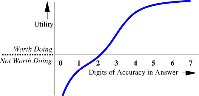
Figure 1. "Utility Curve"
[Note that this is quite different from the
amount of precision that might be required in the computation for typical
algorithms. We have grown so accustomed to the use of 64-bit arithmetic with 14
to 16 decimals of accuracy in the computation that we tend to forget to consider what we need in the
accuracy of the result.]
A
somewhat different model is to define "acceptability," a function bounded by 0
(unacceptable) and 1 (completely acceptable) that is monotone increasing in
some parameter, assuming all other parameters are completely acceptable. Such
curves might be approximated as "logistic curves," which are functions of the
form
A(x) = 1 / (1 + ea + bx) (1)
where b is less than zero.
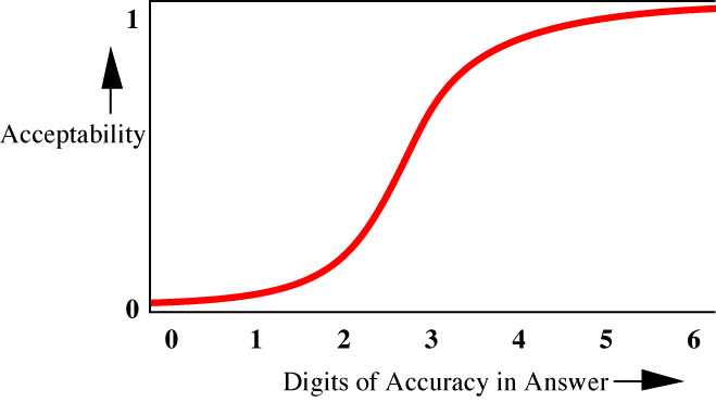
Figure 2. Typical "Acceptability Curve"
Both
the Utility model and the Acceptability model ignore cross terms; for example,
a chemistry application with 100 atoms and only one decimal of accuracy might
be acceptable, but when applied to systems of 3 atoms, only answers accurate to
four decimals will be competitive with research done elsewhere. Where cross
terms are easy to recognize, it may be more useful to plot utility versus some
combination of more than one variable (like, accuracy in decimals times the
square root of the number of atoms).
To
see why each Grand Challenge community needs to come up with its own set of Acceptability
graphs, consider the differences between various groups of scientists regarding
run times.
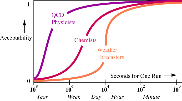
Figure 3. Run time Acceptability Variation by Scientific Culture
From personal observation, QCD physicists
have an extraordinary tolerance for execution times that take a significant
fraction of a human lifetime; they expect to wait months for a single result.
The upper limit of their patience is simply that for runs of more than a year,
computer hardware improvements permit those problems to be started later and
finished sooner. Chemists and most scientists operate more in the range of
several-hour to several-day runs. Weather prediction (not climate prediction)
is clearly limited by the time scale of geophysical events. Outside the Grand
Challenge community, there are computer applications such as text editing where
interactions requiring more than a few seconds are considered intolerable.
If
we are to quantify Grand Challenge goals, we have to include not just the
measures of closeness to physical reality, but the practical demands of the
entire project. There is a tendency to sweep such issues as programming effort
and system up time "under the rug" when measuring computing performance.
Although they are harder to quantify than operation counts or word sizes, they
can be included in the model.
5. THE VARIABLES MOST MODELS LEAVE OUT
Performance studies commonly assume that the only figure of merit one need consider is the reciprocal of the execution time. Putting questions of fixed time versus fixed size scaling for a moment, there are certainly many other things that matter to the computer user, such as:
·
Time for each
edit-compile-run-debug cycle
·
Time to create or convert an
effective simulation program on a particular architecture
·
Initial cost of the system
·
Cost per run, or better, the
cost for a complete solution to the Grand Challenge
·
Probability that any given
run on the computer will fail from reliability problems (hardware or operating
system software)
·
Validity of the answer
(non-obvious failure modes)
Compared
to these issues, the question of how close we get to 1 teraflop/s seems moot.
All of these variables can be made into specific goals by estimating the
Acceptability function and declaring a value at which we declare the subgoal as
"met." The acceptabilities Ai
can be multiplied to form a Composite
Acceptability A = ΠiAi, a bit like
taking the "AND" Boolean operator on all requirements.
The beauty of this approach is that it allows fair comparison of widely varying architectures and algorithms. One is free to change an algorithm to fit a different architecture without worrying about uncontrolled comparisons.
6. EXAMPLE: GRAPHIC RENDERING
The
problem of correctly rendering the appearance of a room defined by the
locations, colors, and reflective properties of its surfaces and lights is a
Grand Challenge in the computer graphics community. What are the requirements
of this challenge?
1)
It should be able to handle
any geometry or reflection property one might find in a typical building
interior.
2)
It should take less than one
minute to compute.
3)
It should cost less than one
dollar for each multi-view rendering.
4)
The time to make a small
alteration to the geometry should be no greater than the time to re-render the
image.
5)
A video display of the scene
should be indistinguishable from a photograph of a real room with the same
geometry. More precisely, it should be within 5% of true luminosity at a display
resolution of 1024 by 1024 pixels, and should have less than 1% chance of
catastrophic failure from any reason.
6)
We want to meet these goals
by the year 2000, with the equivalent of two full-time people working on it.
This
list of goals is not the way the
graphics community has approached the challenge. You will not find such a
specification in the SIGGRAPH Proceedings
or similar literature. Some researchers keep vague goals similar to these in
their head, but the prevailing mode of comparing rendering methods is to
display a picture and show that it "looks realistic." There is seldom any
mention of the mathematical accuracy, the cost of the system that created the
picture, the amount of time spent computing, or the effort to create the
program.
By
expressing these goals, our program at Ames Lab changed its approach to the rendering
problem. Taking each of these goals in turn:
1)
We explicitly restrict
ourselves to surfaces expressible by convex planar quadrilaterals with diffuse
surface reflectivity.
2)
We allow some runs to last
several hours for the sake of prototyping, but otherwise retain this goal.
3)
We retain this goal if one
does not figure in the program development cost or the facilities start-up
costs.
4)
We retain this goal.
5)
We relax this goal by tolerating
about a 10% deviation from correct luminosity.
6)
We are ahead of schedule.
These
compromises can be made more precise using the Acceptability functions of each
goal. One could fit logistic curves to each goal, and then define the product
as the net acceptability. The Acceptability might be a step function for
qualitative requirements like point 1.
Point
5 requires a new formulation of the problem. Normally, diffuse surfaces are
treated using the "radiosity equation":
b(r) = e(r) + r(r) ∫S F(r, r') b(r') dr' (2)
where b is the radiosity (or luminosity) in watts or lumens per meter, r and r' are points
on surfaces in the scene, e is the
emissivity, or light emitted as a source from each point, S is the set of all surfaces, and F is the "coupling factor" that measures the geometric
coupling between points in the scene. For diffuse surfaces, the equation is
exact.
This
is discretized to form a system of linear equations, but here is where the
more explicit goal changed our approach:
We discretize so as to form a rigorous upper bound and lower bound on the
solution. The coupling factor F attains
a maximum and a minimum for any pair of patches i and j, which are
the elements Fijmax and Fijmin of the discretized system
The upper-bound solution can be initially bounded by the maximum light
emissivity emax times the sum of the geometric series for the maximum
reflectivity rmax:
emax (1 + rmax + rmax2 + rmax3 + ...) = emax / (1 - rmax) (3)
The
lower bound solution can be bounded by zero. Both bounds are independent of location
in the scene. Now we subdivide the geometry, keeping careful track of maxima
and minima in the new discretization. The answer is then improved by
Gauss-Seidel iteration without over
relaxation, guaranteeing monotone approach to the correct solution. We alternate
the refining of the subdivision with the iteration of the Gauss-Seidel solver
to tighten the bounds on the answer, producing steady improvement in the
quality of the answer with increased computation. To illustrate this, consider
the simple two-dimensional radiosity problem shown in Figure 4.
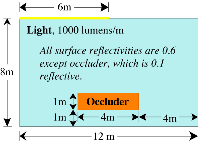
Figure 4. Simple Radiosity Geometry
Figure 5 shows how the true, continuous
solution to the equation is bounded by the discrete form, for a coarse discretization.
The answer "quality" can now be defined as the reciprocal of the total area
between lower and upper bounds.
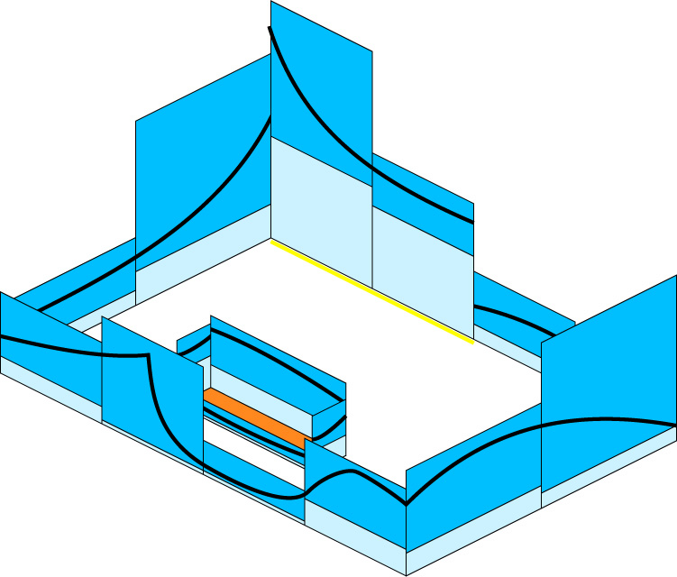
Figure 5. Rigorously Bounded Solution
The
use of rigorous bounds for the answer to a continuum problem seems to be rare.
Computational scientists tend to use double precision and trust that it
represents the true answer except for the last few decimals of a 15-digit
answer. This is seldom a valid approach, since discretization error dominates
most problems. Once we realized there was no point to requiring an error of 10-15 in the solution with 1% error in the
discretization, we were able to make tremendous improvements to our run times.
We are currently running graphics rendering problems that would take over a
thousand times as long using our old paradigm. Stating our goals clearly caused
us to realize that much of our effort was misplaced. A similar approach could
well be used for the federal Grand Challenges.
7. Translating GC
Goals to Hardware Design Goals
Hardware
designers are faced with an ill-defined problem: How does one allocate hardware
costs to maximize performance on a Grand Challenge? The naïve approach of "Make
every component as high performance (which usually means 'fast' or 'large') as
possible" does not work because cost cannot be ignored. Unfortunately, the
"Teraflops" goal has sent the message to designers that nothing matters but
floating point arithmetic speed. Thus, designers are implicitly guided to
provide I/O, memory speed, memory size, ease of use, and MTBF only to the
extent that they affect the nominal flop/s rate. This has had a disastrous
effect on the suitability of many designs for Grand Challenge applications.
Every engineering goal must have subgoals; however, some of our subgoals seem
to be the wrong ones in that they lead us farther from, not closer to, the
ultimate goal.
Some
specifics: A sustained teraflop/s implies a memory size of roughly 1 teraword (not terabyte),
which at 1994 personal computer SIMM prices costs from $250M to $1000M. The
processors capable of a net theoretical performance of 1 teraflop/s, in contrast,
cost under $5M using currently available RISC chips. Why, then, is the flop/s
performance still regarded as the design challenge? It is the least of our
worries.
Balancing
memory bandwidth seems to lead to several pitfalls: belief in caches as a
complete solution, and reliance on benchmarks that involve unrealistic levels
of reuse of data elements (such as matrix multiply). The Level 3 BLAS are
characterized by order n3 operations on order n2 quantities. Such operations are beloved of marketing
departments because they produce high flop/s numbers for advertising claims,
but represent a vanishingly small part of Grand Challenge workloads. A better
design rule would be to test all computer operations on order n algorithm constructs. To do n multiplications as a memory-to-memory operation in 64-bit
precision requires moving 24n bytes to
or from main memory. Hence, a teraflop/s computer should have a nominal total memory
bandwidth of 24 terabytes/s, a daunting figure in 1994. Uncached memory
bandwidth has a strong correlation with computer hardware cost. There is no
free lunch. In 1994, I estimate the cost of memory bandwidth in a balanced
system to be $40 per megabyte/s. The bandwidth for a "sustained teraflop/s"
therefore costs about $100M if scaling is linear (optimistic scaling, but
realistic for distributed memory systems that rely on explicit message
passing).
SUMMARY
We
have used the term "Grand Challenge" to organize our HPCC efforts and justify
support for large-scale computational research. The goal of "a sustained
teraflop per second" is the hardware challenge often mentioned in the same
breath as "Grand Challenge." These goals may not lie in the same direction. To
the extent that we let the measure of operations per second be an end in
itself, we are distracted from the real goal of solving physical problems by
computer. For some specific examples, the goals may even be in opposite
directions; we can achieve higher nominal flop/s rates only by using less
sophisticated algorithms that delay the solution.
If
we define all our performance measures in terms of answer goals, these problems
disappear. We can compare parallel computers with vector computers with serial
computers running all different algorithms without questions of "fairness."
With the improved definition, hardware designers can produce computers better
suited to our needs, and we can use the systems in a way far better suited to
solving the Challenges.
REFERENCES
[1] D. Bailey et al., "The NAS Parallel
Benchmarks," Report RNR-91-002,
NASA/Ames Research Center, January 1991.
[2] J. Gustafson, "The Consequences of Fixed Time
Performance Measurement," Proceedings of the 25th HICSS Conference, Vol. III, IEEE Press, 1992.
[3] W. Pardee, "Representation of User Needs in
Grand Challenge Computation," Special Report by Pardee Quality Methods (805) 493-2610 for Ames Laboratory, 1993.
[4] D. Snelling, "A Philosophical Perspective on
Performance Measurement," Computer Benchmarks, J. Dongarra and W. Gentzsch, editors, North Holland,
Amsterdam, 1993, pp. 97-103.
[5] X.-H. Sun and J. Gustafson, "Toward a Better
Parallel Performance Metric," Proceedings of DMCC6, ACM, 1991.
[6] F. Weingarten, "HPCC Research Questioned," Communications of the ACM, Vol. 36, No. 11, November 1993, pp. 27-29.