Figure 1. SLALOM Performance for
Parallel Product Families
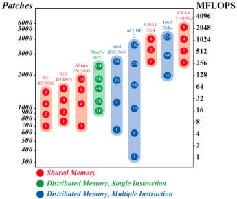
* Note: 400-node Intel Delta results not represented
in chart. See Table 1.
SLALOM
IS YOUR COMPUTER
ON THE LIST?
BY John Gustafson, Diane Rover, Stephen Elbert, and Michael Carter
Eight months ago, when SLALOM was
introduced in Supercomputing Review, we charted the performance of about 20
computers. That list is now approaching 100 entries.
This month we’ll present the actively marketed systems as well as more widely known, older computers. Only Dongarra’s LINPACK list has more entries, and no other benchmark based on complete application measurement has as many machines...or as wide a variety.
The SLALOM list has the Intel Touchstone,
the Macintosh LC, the largest CRAY, the IBM workstations, and the MasPar
data-parallel computers, all under a single comparison. We can compare these
highly disparate architectures using the concept of fixed-time benchmarking: Run the
largest problem possible in under one minute, and use the problem size as the figure of merit.
Some people have said that SLALOM is a parallel computer benchmark. It’s nothing of the kind. In fact, the backsolving of the equations and the writing of the solution to disk are proving to be major challenges for the parallel machines. SLALOM fits any architecture, any language, a very wide range of performance, and any native word size. So yes, it runs on parallel computers. There are at least two dozen entirely different high-performance architectures on the list.
Maybe the most startling news is that, until late-breaking news from Intel, a Japanese-made uniprocessor topped the list. The Siemens S600/20, equivalent to a top-of-the-line Fujitsu model, climbed past the CRAY Y-MP/8. As many people have pointed out, “uniprocessor” might be a misnomer for a machine with enough pipelines to deliver eight multiplies and eight adds every 3.2 nanoseconds! It’s interesting that Japanese computers bracketed the list, with a Fujitsu supercomputer at the top and a Toshiba laptop computer at the bottom.
The Intel iPSC/860 version has been well-tuned by people at the Intel Supercomputer Division in Beaverton, Oregon, and is up to about five MFLOPS per processor. The Touchstone Delta system at Caltech reached 4320 patches, or roughly 1.3 GFLOPS. That run used only 256 of its 512 processors. At the top of the list, the parallel computers continue to threaten, but not overtake, the most expensive vector supercomputers.*
Historical
Note
Sometimes we hear people say, “The only performance figure that matters is how long it takes to run my application.” But, what people say matters to them and how they use higher performance are two different things. It might be more accurate to say, “The only performance figure that matters is the problem size I can solve in the time I’m willing to wait.” Consider the following quotations about computing tasks, taken from historical treatises [4]:
The determination of the logarithm of any number would take 2 minutes, while the evaluation of an (for any value of n) by the expotential [sic] theorem, should not require more than 1 1/2 minutes longer-all results being of twenty figures.
— On a
Proposed Analytical Machine
P. Ludgate, 1878
The work of counting or tabulating on the machines can be so arranged that, within a few hours after the last card is punched, the first set of tables, including condensed grouping of all the leading statistical facts, would be complete.
— An Electric
Tabulating System
H. Hollerith, 1889
Since an expert [human] computer takes about eight hours to solve a full set of eight equations in eight unknowns, k is about 1/64. To solve twenty equations in twenty unknowns should thus require 125 hours... The solution of general systems of linear equations with a number of unknowns greater than ten is not often attempted.
— Computing
Machine for the Solution of Large Systems of Linear Algebraic Equations
J. Atanasoff, 1940
Another problem that has been put on the machine is that of computing the position of the Moon for any time, past or future ... Time required: 7 minutes.
— Electrons
and Computation
W. J. Eckert, 1948
…13 equations, solved as a two-computer problem, require about 8 hours of computing time. The time required for systems of higher order varies approximately as the cube of the order. This puts a practical limitation on the size of systems to be solved ... It is believed that this will limit the process used, even if used iteratively, to about 20 or 30 unknowns.
— A Bell
Telephone Laboratories Computing Machine
F. Alt, 1948
Tracking a guided missile on a test range ... is done on the International Business Machines (IBM) Card-Programmed Electronic Calculator in about 8 hours, and the tests can proceed.
— The IBM Card-Programmed Electronic
Calculator
J. W. Sheldon and L. Tatum, 1952
Computer speeds have increased by many orders of magnitude over the last century, but human patience is unchanging. The computing jobs cited in publications typically take from minutes to hours, whether the technology is pencil-and-paper, gears, vacuum tubes, or VLSI. Pick any fixed-size benchmark, and it will soon be rendered obsolete by hardware advances that make the benchmark absurdly small. People tend to forget the numerator in the ratio that defines the “speed” of computing. Give a scientist a faster supercomputer, and he or she will use it to solve a new, larger problem… not to reduce the execution time of last year’s problem.
A Scalable Benchmark
for Scalable Computers
A given make of parallel processor can offer a performance range of over 8000 to 1, so the scaling issue exists even if applied to a computer of current vintage.
It’s not easy to use conventional benchmark techniques on every possible size of a large parallel ensemble like an nCUBE or an Intel. In papers on such computers, you’ll see footnotes like, “We were unable to run the problem on small numbers of processors because of insufficient memory.” Or the performance graph is graphed with a collage of partial curves, each for a particular problem size.
The fixed-time method simplifies the issue by changing the question. None of the machines in our database has had insufficient memory to run for one minute, since the memory scales with the speed.
As Figure 1 shows, SLALOM can easily compare computers that scale by 1024-1. You might have seen charts like Figure 1 before for nominal MIPS or MFLOPS rates, but this chart is for a complete application. (SLALOM times a real radiation transfer problem, including input/output and setup tasks. The “patches” number determines the answer resolution.)
Figure 1. SLALOM Performance for
Parallel Product Families
* Note: 400-node Intel Delta results not represented
in chart. See Table 1.
The fixed-time benchmark concept is not the same as generic rate comparisons, such as “transactions per second,” “logical inferences per second,” or “spin updates per second.”
In fixed-time performance comparison, a complete computing job is scaled to fit a given amount of time, whereas rate comparisons use the asymptotic speed of a supposedly generic task.
As with MFLOPS or MIPS metrics, generic rate comparisons are usually vague in defining the unit of work. Floating-point operations, instructions, transactions, logical inferences, and spin updates come in many different sizes and varieties. True fixed-time benchmarking considers the entire application. A complete application usually contains many different work components with different scaling properties.
There are now 82 computer systems in the
“Actively Marketed” list that follows. To save space, we give only the briefest
description of the system and the environment used. The list ranks computers by
the size of the problem they could run, not MFLOPS. The MFLOPS are estimated
from the best serial algorithm known at the time of the run, and are
approximate. All runs are very close to 60 seconds, so we don’t list execution
times.
S calable
L anguage-independent
A mes
L aboratory
O ne-minute
M easurement
NOTES:
A
“(v)” after the name of the person who made the measurement indicates a vendor.
Vendors frequently have access to compilers, libraries, and other tools that
make the performance higher than that achievable by a customer.
Intel
entries for 8 and 32 nodes used a one-dimensional scattered decomposition;
other Intel and nCUBE entries used a two-dimensional scattered decomposition
that currently works only for even-dimensioned hypercubes.
The
IBM RS/6000 workstations were not all measured using the same algorithm. Be
careful not to compare machines submitted on different dates even when all
other information is identical. A recent improvement to the SetUp routines by
J. Shearer allowed the 25 MHz model 530 to surpass the older algorithm on a 30
MHz model 540.
If
MFLOPS seem inconsistent with preceding/following entries, it is because either
the number of seconds is significantly less than 60 or a different version of
the algorithm was used. Operation counts are reduced as more efficient methods
are found. Rankings are by patch count, not MFLOPS.
 Most Wanted List
We
haven’t heard from everyone yet. Our “most wanted” computers in the SLALOM
table include those made by the following vendors:
We hope to add these and
other computers to our list by our next publication in Supercomputing Review.
Performance
within a product line
Here’s another way to look at some entries on our list. We’ve chosen those computers for which at least three different numbers of processors have been measured, and grouped them by type. The groups are sorted in descending order of the speed of their fastest member. This is the same data shown graphically in Figure. 1.
The “speedup” column is the ratio of the
MFLOPS rate to that of the smallest member of the product line for which we
have SLALOM measurements. Since MFLOPS are a poor method of assessing
performance, the speedup column should be viewed only as a rough guide to the
scalability of a product line via parallel processing. This form of speedup can
be greater than the number of processors because faster computers spend a
greater fraction of the time on the Solver, raising the MFLOPS rate per
processor. This “changing profile” effect, noted in past SLALOM reports, tends
to compensate for the increasing communication and load imbalance that result
from using more processors.
Table 2. The SLALOM Report — Selected Product Families
From time to time, we will publish lists of SLALOM performance for computers that are no longer actively marketed. We feel that current and historical computers should not be mixed in the same list, so we intend to move entries from the main list to this one when we learn that a particular model has been superceded or is no longer available from the original vendor.
Table 3. The SLALOM Report — Older Computers
Acknowledgments
We thank everyone who has participated in this effort. In particular, analysts at Alliant, Cogent, Cray, IBM, Intel, MasPar, and Myrias have contributed suggestions, ideas, and versions of SLALOM. Much of the work was performed at the Scalable Computing Laboratory at Ames Laboratory/Center for Physical and Computational Mathematics.
1. V. Faber, O. Lubeck, and A. White,
“Superlinear Speedup of an Efficient Sequential Algorithm is Not Possible,” Parallel
Computing,
Volume 3, 1986, pages 259–260.
2. J. L. Gustafson, “Reevaluating
Amdahl’s Law,” Communications of the ACM, Volume 31, Number 5,
May 1988.
3. D. P. Helmbold. and C. E. McDowell,
“Modeling Speedup(n) greater than n,” 1989 International Conference on Parallel
Processing Proceedings, 1989, Volume III, pages 219–225.
4. D. Parkinson, “Parallel Efficiency can be
Greater than Unity,” Parallel Computing, Volume 3, 1986, pages 261–262.
5. B. Randell, editor, The Origins of
Digital Computers: Selected Papers, Second Edition, Springer-Verlag, 1975, pages
84, 138, 227, 229, 283, and 306.
* This work is
supported by the Applied Mathematical Sciences Program of the Ames
Laboratory-U.S. Department of Energy under contract number W-7405-ENG-82.