The Design of a Scalable, Fixed-Time Computer
Benchmark

John Gustafson, Diane Rover, Stephen Elbert, and Michael Carter

Abstract

By using the principle of fixed-time benchmarking, it is possible to compare a wide range of computers, from a small personal computer to the most powerful parallel supercomputer, on a single scale. Fixed-time benchmarks promise greater longevity than those based on a particular problem size and are more appropriate for “grand challenge” capability comparison. We present the design of a benchmark, SLALOM, that adjusts automatically to the computing power available and corrects several deficiencies in various existing benchmarks: it is highly scalable, solves a real problem, includes input and output times, and can be run on parallel computers of all kinds, using any convenient language. The benchmark provides an estimate of the size of problem solvable on scientific computers. It also can be used to demonstrate a new source of superlinear speedup in parallel computers. Results that span six orders of magnitude for contemporary computers of various architectures are presented.

1. INTRODUCTION

Computer power has increased over 70% per year for the last 50 years, or over 11 orders of magnitude. This increase makes it difficult to measure performance with a tool that does not scale. Consider the following quotations concerning examples of computing tasks, taken from historical treatises on computing [12]:

The determination of the logarithm of any number would take 2 minutes, while the evaluation of a_n (for any value of n) by the expotential theorem, should not require more than 11⁄2 minutes longer – all results being of twenty figures. (On a Proposed Analytical Machine, P. Ludgate, 1878)

The work of counting or tabulating on the machines can be so arranged that, within a few hours after the last card is punched, the first set of tables, including condensed grouping of all the leading statistical facts, would be complete. (An Electric Tabulating System, H. Hollerith, 1889)

Since an expert [human] computer takes about eight hours to solve a full set of eight equations in eight unknowns, k is about 1/64. To solve twenty equations in twenty unknowns should thus require 125 hours… The solution of general systems of linear equations with a number of unknowns greater than ten is not often attempted. (Computing Machine for the Solution of large Systems of Linear Algebraic Equations, J. Atanasoff, 1940)

Another problem that has been put on the machine is that of computing the position of the moon for any time, past or future… Time required: 7 minutes. (Electrons and Computation, W. J. Eckert, 1948)

…13 equations, solved as a two-computer problem, require about 8 hours of computing time. The time required for systems of higher order varies approximately as the cube of the order. This puts a practical limitation on the size of systems to be solved… It is believed that this will limit the process used, even if used iteratively, to about 20 or 30 unknowns. (A Bell Telephone Laboratories Computing Machine, F. Alt, 1948)

Tracking a guided missile on a test range… is done on the International Business Machines (IBM) Card-Programmed Electronic Calculator in about 8 hours, and the tests can proceed. (The IBM Card-Programmed Electronic Calculator, J. W. Sheldon and L. Tatum, 1952)

These examples document the unchanging scale of human patience. The computing jobs cited in publications typically take from minutes to hours, independent of the speed of the computer involved. Any benchmark of fixed size is soon made obsolete by hardware advances that render the time and space requirements of the benchmark unrepresentative of realistic use of the equipment. The common workaround of performing the undersized task repetitively is less than satisfactory. Furthermore, a given make of parallel processor can offer a performance range of over 8000 to 1, so the scaling problem exists even if applied to a computer of current vintage.

A related issue is the difficulty of scientifically comparing computers with vastly different architectures or programming environments. A benchmark designed for one architecture or programming model puts a different architecture at a disadvantage, even when nominal performance is otherwise similar. Assumptions such as arithmetic precision, memory topology, and “legal” language constructs are invariably wedded to the job to be timed, in the interest of controlling as many variables as possible. This “ethnocentrism” in benchmark design has hampered the comparison of novel parallel computers with traditional serial computers. Examples of popular benchmarks that have some or all of the foregoing drawbacks are LINPACK [3], “PERFECT Club” [11], Livermore Loops [9], SPEC [15], Whetstones [2], and Dhrystones [17].

Section 2 presents the design goals of a benchmark that attempts to solve these and other difficulties. Section 3 shows our techniques for achieving these goals. Section 4 discusses fixed-time profiling and implications of the fixed-time method for superlinear speedup. Section 5 gives experimental results for a wide range of parallel and serial computers.

2. PERFORMANCE MEASUREMENT GOALS

Ideally, a benchmark should be scalable, broad in architectural scope, simple to apply and understand, representative of the way people actually use computers, and scientifically honest. A proper benchmark is both a task engineered to meet these goals and a set of rules governing the experimental procedure. It is more than just an application program or excerpt. We recognize that many of these goals are at odds with one another. As with any engineering design, a certain amount of compromise is necessary.

In particular, a single benchmark with a single figure of merit cannot fully characterize performance for the entire range of computing tasks. We make no pretense of having solved this difficulty. Although we present a particular fixed-time benchmark here, our intent is to illustrate the fixed-time technique as a general principle that should be applied to a variety of computing tasks to obtain a better picture of overall performance. However, it seems possible to restrict ourselves to large-scale scientific problems and capture salient features of that class of problems that are absent from other computer performance tests.

2.1. Goal: Scalable Benchmarking

It is a natural assumption that in measuring computer performance the problem being solved is fixed as the computing power varies. Unfortunately, this is a dubious assumption since it does not reflect the way people actually use computers. Generally, problems scale to use the available resources (both memory and speed), such that the execution time remains approximately constant [1, 6, 7, 18].

The problem of solving systems of linear equations is a scalable one, and one central to scientific computing. The first electronic digital computer, designed by Atanasoff in 1933–1939, was intended to solve a dense linear system of 29 equations in 29 unknowns [12]. When the LINPACK software was first introduced, timings for solving a 100 by 100 system were gathered from a number of institutions and published. In 32-bit precision, the problem only required 40,000 bytes of storage and about 670,000 floating-point operations. A computer such as a VAX-11/780 took several seconds for the computation—a short but plausible amount of time to wait for an answer. As computers have increased in size and speed, the 100 by 100 problem has become increasingly inappropriate for measuring high-speed computers. The CRAY Y-MP8/832 performs that problem in less than 1⁄300 of a second, faster than almost any display can refresh to inform the user that the task is done. Even in 64-bit precision, the CRAY uses less than 1⁄30,000 of its main memory for such a problem. As a result, a new version of the benchmark was introduced for a 300 by 300 problem. When this also began to look small, a 1000 by 1000 version was added. Variations for precision and allowable optimizations have further multiplied the number of meanings of the phrase “LINPACK benchmark.” The LINPACK benchmark has limited scalability even as a kernel, since its random number generator produces singular matrices for large matrix sizes. In fact, no major benchmark in use before 1990 has been designed for scalability.

Yet, most real scientific problems are inherently scalable. We use n here to indicate some measure of both problem size and difficulty. It need not be tied to instruction counts or floating-point operations or bytes of storage; it should simply increase with the quality or complexity of the simulation. For example, scientific problems often involve n degrees of freedom, where n is variable over a wide range depending on the accuracy and realism desired. We seek such a problem as the basis of the benchmark. By varying n, the benchmark should be able to track changes in available performance.

We also wish to allow n to vary on a fine scale. That is, the problem should accommodate any integer n above some threshold and not, for example, restrict n to perfect squares or powers of 2. This allows the exploration of the space of problem size versus number of processors in detail, for parallel systems with adjustable numbers of processors.

2.2 Goal: Fixed-Time Benchmarking

Rather than fix the size of the job to be run, we wish to fix the time and scale the work to be done to fit within that time. A time of 1 min is used in our current effort, but any time range within the limits of human patience (about 0.1 s to 1 month) for a single computer task could be used as the constant. Shorter times do not fully exercise a system, and longer times are tedious and expensive to use as a benchmark. The benchmark should time itself and adjust the problem size automatically for the specified time, or allow the user to search manually. We wish to consider only elapsed time, not “CPU time,” or other subsets of what the user perceives.

An important consequence of the fixed-time model is that “Amdahl’s law” loses its relevance and its predictive powers in understanding the limits to vectorization, parallel processing, and other architectural ideas [6, 7]. We feel that this “fixed-time” approach should be used in benchmarking computers generally. The approach can also serve as a guide to the computer designer estimating the performance gains that might be obtained from architectural enhancements.

It is important to note that the fixed-time model is distinct from the “scaled speedup” model, in which the problem size, as measured by the storage of variables, is scaled with the number of processors [7, 16]. On ensemble computers, simply replicating the problem on every processor will usually make total execution time increase by more than just the cost of parallelism. Fixing work per processor instead of storage per processor keeps run time nearly constant. A simple example is that of matrix factoring.

Consider the simple problem of solving n equations in n unknowns, with full coupling between equations (dense matrix representation). Arithmetic work varies as n³, with storage varying as n². On a P-processor distributed memory system, simply replicating the storage structures on every processor will not generally lead to a fixed run time, since the arithmetic work to solve a matrix with Pn² elements is P^3/2n³, whereas a fixed time model that assumes negligible parallel overhead on P processors would call for Pn³ arithmetic work. This means that the scaled model execution time increases as P^1/2.

This situation appeared in the wave mechanics, fluid dynamics, and structural analysis problems run on the 1024-processor hypercube at Sandia [7], which similarly involved order O(n²) data storage and O(n³) arithmetic complexity. On the 1024-processor hypercube, to simulate a like amount of physical time (or convergence accuracy for the structural analysis problem) took about 1024^1⁄2 = 32 times as much ensemble computing time. It was then that we realized that the historical “just make the problem larger” argument for distributed memory might be simplistic to the point of being fallacious. The scaled model is still the best one to use if storage rather than time dictates the size of the problem that can be run, but the fixed-time model more realistically limits the extent to which problem scaling can be used to reduce communication cost for ensemble computers.

For these “n²– n³” problems, it is useful to think about increasing the ensemble size by powers of 64. With 64 times as much computing power, increasing n by a factor of 4 increases the work by a factor of 4³ = 64, which should keep execution time about constant if parallel overhead is low. However, the total data storage then increases only by a factor of 4² = 16, not 64. Thus, each processor actually decreases in local storage requirements by a factor of 4. With the typical distributed memory approach of using subdomains on each processor, the subdomain dimensions shrink by 50% for every factor of 64 increase in the number of processors. Fixed-time performance models must reduce the size of subdomains as the number of processors P increases, if work grows faster than storage. For the n²– n³ problems, the linear size m of an m by m subdomain will vary as P^–1/6 if we assume linear performance increases. On a log–log graph of problem size and ensemble size, the ideal fixed-time model appears as a line of slope 2⁄3, the ratio of the exponents for storage complexity and work complexity (see Fig. 1).

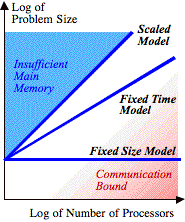
FIG. 1. Problem size vs. ensemble size.

2.3. Goal: Language/Architecture Independence

Rather than define the task with a particular program written in some language, the problem to be solved should be specified at a more abstract level. A benchmark should state what is to be computed for a given range of possible inputs, but not how to compute it. The range of possible inputs should be large enough that major deviations from running some form of the basic algorithm (such as looking up the answer in a large precomputed table) are not practical. This helps to control one experimental variable: the particular algorithms being compared. Any version of the benchmark that arrives at correct answers for the full range of possible inputs, without artificial binding to language or architecture, should be permitted. Significant departures from established algorithms should be published along with the resulting performance.

A benchmark should be able to exercise new architectural concepts as they arise, such as massive parallelism. We are most interested in the use of powerful computers to simulate physical systems. Since most physical systems have ample parallelism, use of a physics-based problem should provide a way for parallel computers to demonstrate their capabilities. An example of a trivially parallel problem is multiple runs with different starting assumptions. An example of an inherently serial problem is the 3-body problem for a large number of time steps. Both trivial parallelism and inherent serialism should be avoided as extreme cases of serial/parallel ratios that are not representative of mainstream scientific computing.

2.4. Goal: Precision Independence

Rather than specify an arithmetic precision to be used, such as “64-bit IEEE floating-point arithmetic,” self-consistency should be required in the result to a certain relative error. The user is then free to achieve a result within that tolerance using any calculation method or precision. The rules for precision should be determined by the desired precision in the result, not by dictating the method of calculation. Physical conservation laws are very helpful in testing self-consistency in scalable problems.

2.5. Goal: Valid Figure of Merit

Performance evaluation is inherently multidimensional. Yet, efforts to disseminate statistical information have not been very successful. The Livermore Loops present 24 speeds for three different vector lengths, with a variety of ways to sum and average the results, and yet one sees statements like “Our computer runs the Livermore Loops at 10.8 MFLOPS.” The SPEC benchmark also contains 10 components of widely varying nature (from matrix kernel operations to a complete circuit simulation), yet the “SPEC mark” is the oft-quoted scalar quantity derived from these components. Recognizing this unfortunate tendency, we seek to produce a single figure of merit number that is meaningful [14]. We should supplant this with multidimensional information in the form of built-in profiling that allows one to see the time spent for input/output, scalar routines, vector routines, etc., that can provide insight into the reasons behind the “one-number” summary.

Instead of using questionable performance measures such as MIPS (Millions of Instructions Per Second), or MFLOPS (Millions of Floating-Point Operations Per Second), the basis of comparison should be simply n, the problem size. Although other work measures can be provided by the benchmark as a guide to optimization, they are not the coin of the realm. A computer should be considered more powerful than another on a fixed-time benchmark if and only if it runs a “larger” (bigger value of n) problem in the time allotted. It is not necessary that work be a simple function of n (and it seldom is), but the work should be a strictly increasing function of n. The value of n cannot be used as a direct measure of performance in the sense of cost efficiency. A computer that achieves a value of 2n is not, in general, “twice as powerful” as one that achieves a value of n.

2.6. Goal: Complete Task Measurement

With a fixed-time paradigm, it becomes practical to include costs such as disk input/output and the setting up of equations to be solved. Since computers tend to improve to balance speeds with fixed time rather than fixed-size jobs in mind, these previously excluded components of computer use can be fairly included in the measurement. We strongly feel that it is incorrect to test only the compute-intensive part of a task. Even recent efforts such as the PERFECT and SPEC test suites excise the input and output functions in some or all of their component routines [11, 15].

2.7. Goal: Minimization of Human Effort Bias

Since converting programs to different architectures imposes a burden that is reflected (at least temporarily) in reduced performance, the benchmark should be disseminated in as many representative forms as possible: traditional, vectorized, shared memory parallel, distributed memory parallel, etc. It should also be maintained in many languages such as C, Fortran 77, Pascal, and Fortran 90, to reduce language conversion effort. In the sense that computer benchmarks compare programmers as well as computers, a centralized and collective body of conversion tools makes the comparison fair and deemphasizes programming skill. For the same reason, great effort should be put into finding the “best serial algorithm,” that is, the solution method with the smallest apparent complexity. Otherwise, a problem thought to be some complexity like O(n³) might later prove to be O(n² log n), which only some programmers would discover and exploit.

2.8. Goal: Accountability

For some reason, virtually all published benchmark data delete the source of the data. In contrast to scientific reporting, computer benchmark figures are seldom accompanied by the name of the person who ran the benchmark and the date that the figures were submitted. To preserve the integrity and accountability of the comparison, the benchmark should include these data, along with the institutional affiliation of the person submitting the measurement.

3. DETAILED DESCRIPTION

The following sections amplify the preceding ideas. The Scalable, Language-independent, Ames Laboratory One-minute Measurement (SLALOM) was created to meet the objectives described above.

3.1. Scalable Benchmarking

In September 1989, we began a search for a complete, practical scientific problem that demands the solution of a set of n fully coupled equations similar to the traditional LINPACK test. Conventional methods for such problems require O(n³) operations for solution and O(n²) operations for setup. Storing the answer, a list of n numbers, takes O(n) operations. Reading a description of the geometry and other physical parameters of the problem takes O(1) operations. The memory required for the problem varies as n². These scaling characteristics capture the salient features of a wide spectrum of scientific computing tasks. With careful design of the problem discretization, n can be chosen as any positive number, to permit fine adjustment of the work and storage needed.

Most scientific problems involve systems of equations that are sparse, symmetric, and diagonally dominant. This contrasts with the benchmark tradition of dense, nonsymmetric systems requiring partial pivoting. We have been unable to find a genuine scientific problem for which the best-known algorithm requires the direct solution of a nonsymmetric, dense matrix with partial pivoting. Therefore, we abandon the tradition of testing such an obscure variety of matrix problem and seek a problem closer to the mainstream. We attempt to preserve some continuity with previous benchmarks by looking for a problem that is nearly dense, such that the innermost basic linear algebra operations are the same as for the well-studied dense case. We acknowledge that this is a compromise and may move to very sparse systems in our future benchmark efforts.

A diagonally dominant nearly dense matrix problem can be found in the pioneering paper by Greenberg, Goral, et al. on “radiosity” [5], which is the equilibrium radiation given off by a coupled set of diffuse surfaces that emit and absorb radiation. The problem is easily described and understood: A room is painted with a separate color for each wall, plus floor and ceiling, and one or more of the six surfaces emits light.

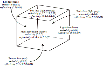
FIG. 2. Radiosity in a box.

Emissivity and reflectivity are described as red–green–blue components for each wall of the room. The problem is to find the color variation over each wall. Goral’s paper uses an example test case as shown in Fig. 2, with unit face sizes. There is a white, light-emitting ceiling, shades of gray on the floor, front, and back walls, and saturated red and saturated blue side walls. (We usually use the term “face” instead of “wall,” and “box” instead of “room,” in this paper.) With diffuse surfaces, there is a “bleeding” of color to nearby surfaces.

Goral’s paper offers limited scaling, breaking each face into 3 by 3, 5 by 5, and 7 by 7 “patches,” with 6m² equations to solve for an m by m patch decomposition. The coupling between patches is the “fraction of the sky” that each patch “sees” occupied by another patch, for which the Goral paper uses an approximate quadrature.

We coded the radiosity problem in a scalable fashion, to allow any number of patches n, from six on up. The challenge is to write an automatic decomposition algorithm that is both concise and amenable to parallel processing, so the process will be treated in some detail here. The initial approach was to assume that the box is a unit cube, find the largest m such that 6m² is less than n, and then halve patches until n was reached. For example, for n = 27 patches, one would start with ë√(27⁄6)û = 2 for m, and then split three patches in two (see Fig. 3).

FIG. 3. Initial attempt at scalable decomposition.

This simple approach worked, but with drawbacks. It created patches of very different areas, implying uneven accuracy in the numerical solution. A practical program would more likely seek to reduce the maximum error by keeping patches as similar in area as possible. Furthermore, the regularity of such a decomposition encourages a clever programmer to shortcut coupling calculations by noticing that many pairs of patches have the same spatial relationship (see Fig. 4).

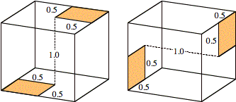
FIG. 4. Examples of exploitable symmetries.

In addition, the solution for a perfect cube is too special to resemble a practical radiosity calculation. Hence, we allow variable box dimensions, restricted to the range 1–100 length units, and decompose the surface of the box into patches that are as nearly square and as nearly equal in area as possible. Exploitation of repeated geometric relationships becomes much more difficult, accuracy for a given number of patches is improved, and the problem more closely resembles a real problem for which a scientific computer might be used.

Let A_i be the area of face i, and A be the total area. Then we want

Number of patches on face i ≈ n ´ A_i / A.

Actually, we mark “start–end” patch numbers for each face. Face 1 starts with patch 1; face 6 ends with patch n. In between, face i starts with the patch that face i–1 ended with, plus one. Face i ends with patch ë∑A_j /A + 0.5û, where the summation is j = 1 to i. The “ë…+ 0.5û” technique explicitly rounds to the nearest integer, breaking ties by rounding up. This explicitness was discovered to be necessary when we tested language independence between Fortran and Pascal, since implicit rounding functions in Pascal use round-to-nearest-even rules, whereas Fortran uses round-toward-zero rules.

Within a face, we desire patches that are as nearly square as possible, to reduce discretization error. This is accomplished by dividing each face first into columns, with the number of columns given by ëÖ(patches/eccentricity) + 0.5û. The eccentricity is the ratio of the face dimensions. For example, to put seven patches on a 2 by 3 face, use ëÖ(7 / 3⁄2) + 0.5û = 3 columns. We can slightly increase robustness by using one column when this formula gives zero columns for a face. However, there must still be an error trap for the case of no patches on a face. For example, a 1 by 1 by 50 box with only six patches will decompose to having no patches on the 1 by 1 faces (each being only 1⁄200 of the surface area) and the benchmark must signal a need for more patches for such a problem.

Let n_patch be the number of patches on a face and i be the local number of a patch on that face, 1 ≤ i ≤ n_patch. Let n_col be the number of columns on the face, as determined by the preceding discussion. Then patch i resides in the column given by

i_col = ë(i – 1) ´ n_col / n_patch û + 1 (1)

for arrays with index origin 1. Note that 1 ≤ i_col ≤ n_col. This assignment of patches to columns distributes “remainder” patches (that is, those in excess of an exact integer division of n_patch by n_col) evenly across the face rather than clumping them at one extreme. A geometrical interpretation of the subdivision for n_patch = 7 and n_col = 3 is shown in Fig. 5.

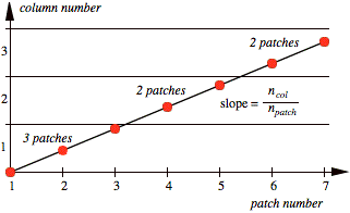
FIG. 5. Column number vs. local patch number.

We can invert (1) to find the range of i for a given value of i_col:

i_col – 1 ≤ (i – 1) ´ n_col / n_patch < i_col

Û ( i_col – 1) ´ n_patch / n_col + 1 ≤ i < i_col ´ n_patch / n_col + 1

Since the left and right bounds are non-integer in general, use floor and ceiling functions to sharpen the range:

é(icol – 1) ´ npatch / ncolù + 1 ≤ i ≤ ëicol ´ npatch / ncol + 1û (2)

where the ceiling function én / mù is calculable from ë(n + m – 1) / mû, a more language-independent construct. It now follows that the number of rows in a given column is

nrow = éicol ´ npatch / ncolù – é(icol – 1) ´ npatch / ncolù (3)

which gives nrow = {3, 2, 2} for icol = {1, 2, 3} for the example shown in Fig. 5.

Figure 6 shows a solution for the benchmark problem for a 512-patch decomposition.

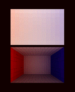
FIG. 6. Example of radiosity solution.

This completes the solution to the scalability problem with respect to domain decomposition. For any problem of size 6 or greater, the preceding method decomposes the benchmark task in a reasonable, portable, concise, numerically sound manner. For a parallel ensemble, the geometry of any subset of the patches can be computed directly from the number of the patch, removing a potential serial bottleneck.

3.2. Fixed-Time Benchmarking

The fixed-time benchmark concept is sometimes confused with generic rate comparisons, such as “transactions per second,” “logical inferences per second,” or “spin updates per second.” In fixed-time performance comparison, a complete computing job is scaled to fit a given amount of time, whereas rate comparisons use the asymptotic speed of a supposedly generic subtask. As with MFLOPS or MIPS metrics, generic rate comparisons are usually imprecise in defining the unit of work in the numerator. Floating-point operations, instructions, transactions, logical inferences, and spin updates come in many different sizes and varieties. True fixed-time benchmarking considers the entire application, which will contain many different work components with different scaling properties.

It is possible to make any scalable benchmark into a fixed-time benchmark simply by putting an upper time bound in the ground rules of the benchmark. If a user-written program can time its own execution, the program can scale itself to run in a specified time. Just as a recursive program operates on its own output, the fixed-time driver creates a benchmark that operates on its own performance. The number to adjust is an integer, n, that describes the “size” of the problem in some sense. Here, n is the number of patches in a radiosity problem, but the technique is general.

The user is asked by the program to supply a desired time interval, which we call goal. (We have found, by experiment, that 60 s is a good compromise between realistically long run times and convenient short times, but the goal time is arbitrary.) The user is then asked to supply a value of n such that the program will take less than goal time to execute.

The program tests that n is within limits imposed by the problem and the computer. For example, the radiosity problem requires n ≥ 6. (If the box is highly eccentric, the minimum n could be larger.) If n passes as a valid lower bound, the timer is started and the benchmark is run. If the benchmark fails to run in less time than goal, the driver repeats its request until a satisfactory lower-bound n is supplied. If it succeeds, the n is saved and the driver proceeds to the next step.

The next stage is to find an n such that the run time is greater than or equal to goal. This simplifies the root-finding procedure by restricting the search space to an integer interval. The reason for disallowing equality with goal is that equality might reward low-resolution timers. For example, a computer capable of self-timing only to 1 s resolution might run 60.999 s, report it as 60 s, and thus be able to run a larger n than a computer with a more precise clock. The effect is admittedly minor, but simple to eliminate.

If goal is large, n might exceed the value allowed by the computer memory allocated by the program being benchmarked. If the n supplied as an upper bound fails to equal or exceed the goal time, the driver repeats its request until a satisfactory n is supplied. The user is responsible for altering the benchmark to allow sufficiently large n, even if it means explicit management of mass storage. Running out of memory to achieve a 1-min SLALOM run might be interpreted as a symptom of unbalanced or special-purpose computer design. Of the 70 computers we have tested, all have had sufficient main memory for a 1-min run.

Note that a given computer might not be powerful enough to run even the minimum n permitted by the benchmark in goal time. We have chosen the problem and goal such that virtually every programmable machine currently marketed is sufficiently powerful to qualify, although computers from a few years ago might not.

With an upper bound and a lower bound, the problem of finding the n that is as large as possible without requiring time greater than or equal to goal is a classic root-finding problem. The time is not necessarily an increasing function of n, nor is it particularly “smooth” for most computers. Pipeline lengths, cache sizes, and memory organization can complicate performance enough to destroy monotonicity. Methods such as Newton–Raphson iteration were tried and found non-convergent in general, for the preceding reason.

There might also be random timing variation for any single value of n. If the variation is greater than the difference in timing for values of n differing by unity, then the n determined by the driver will be a random variable. Intuitively, the distribution of n is zero above some integer, since the hardware has inherent limits (Fig. 7). Hence, we look at the record largest n achievable over any desired number of tests to again reduce the measurement to a single integer value.

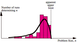
FIG. 7 Distribution of n.

A convergent method that is used in the current version of the benchmark driver is the half-interval method: while n_upper – n_lower > 1, find n_mean = ë(n_upper + n_lower) / 2û. Time the benchmark for n_mean; if it is less than goal, replace n_lower by n_mean and repeat. Otherwise, replace n_upper by n_mean and repeat.

Once n_upper – n_lower = 1, the desired n is n_lower. A problem with this method is that random fluctuations in the timing might assign a particular n as below goal on one run, but above it on the next. Currently, our workaround is to refer to the instance where the execution time was below goal and use that run as the result. We ignore the “final” report of an n value if it equals or exceeds goal.

The fixed-time driver has been developed for several computers and written in several languages. It works satisfactorily in most cases. Random fluctuations can cause it to miss the largest possible n. It can also fail if execution time is not an increasing function of n. Caching and memory bank conflicts, for example, can create “saw tooth” patterns in the execution time that require the operator of SLALOM to revert to manual selection of n.

3.3. Language/Architecture Independence

Two approaches are used to remove ties to a particular language or architecture: a high-level problem specification and a multiplicity of working examples covering a wide spectrum of environments.

A high-level problem specification is practical if guidance is supplied as to what appears to be a “good” solution method, and if the input/output is specified so as to rule out unrealistic use of pre-computed answers. Supplying guidance is like an athletic competition; although certain techniques are known to be effective, competitors may choose what works best for them individually. Advances in technique that appear general are made publicly known as quickly as possible to eliminate an advantage based on disparate knowledge. If only a single input and output are specified, a benchmark with such liberal rules quickly degenerates into the trivial recall of pre-computed answers. However, if input is not specified, run times will vary with input (in general) and thus introduce an uncontrolled variable. The solution is this: the program must work for a specified range of inputs and must time an input (supplied as standard) using the same method as that used for arbitrary input. Stated another way, the program cannot contain any information specific to the standard case.

For the radiosity problem, the standard case is much like the example in Goral’s paper [5] shown in Fig. 2. The main changes are to make the faces rectangular (13.5 by 9 by 8) rather than square and to derive the coupling with exact analytic expressions instead of approximate quadrature. The matrix formulation and solution are similar, except that we divide the matrix row entries by the area of the patch to which they pertain, which renders the matrix symmetric. The discovery that the radiosity problem could be made symmetric, cutting solution time almost in half for large problems, was a surprise to us. It reduces the resemblance of SLALOM to the LINPACK benchmark, but one could argue that symmetric systems of equations are the rule rather than the exception in physical simulations.

As of this writing, we have converted the high-level description of the radiosity problem, as supplied by Goral’s paper, into the following forms:

· Fortran 77

· C for UNIX-based computers

· Pascal

· BASIC (both interpreted and compiled)

· C extended with variables for data parallel computers

· Vectorized Fortran with parallel compiler directives for shared memory parallel computers

· Fortran with message-passing constructs for hypercubes.

We maintain the versions under the SCCS revision control system.

3.4. Precision Independence

We feel that the goal should be to compute an answer within a specified tolerance of the correct answer and not specify the word size or anything else about how to get to that level of precision. The precision needed depends on problem size, although 64-bit floating-point arithmetic suffices for the range measured to date. We hope to eventually run experiments with computing hardware that allows an arbitrary number of bits of precision to find the relationship between arithmetic precision and the error in the result.

The benchmark has two self-consistency checks. One is inside the timed part of the benchmark, since the check is also used to improve the accuracy of the answer if within tolerance limits. The other is a pass-fail verification after the computation is done, not timed. It is very unlikely that an incorrect program will pass both tests, and experience has confirmed this. (We also use comparison of output files and examination of graphic displays of the output as a convenient way to check program correctness for small problems).

The first self-consistency check involves the matrix setup. Let f_ij = the fraction of the hemisphere taken up by patch j, as seen from patch i. For example, f_ij ≈ 1 for close, parallel planes, about 0.2 for unit squares a unit apart or perpendicular and touching, and near 0 for patches that are small relative to their separation (Fig. 8).

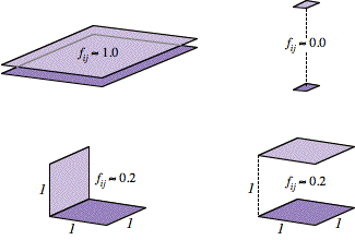
FIG. 8. “Form factor” examples.

These f_ij are variously called “form factors” or “coupling factors” or “shape factors” in the radiation transfer literature. Analytic means exist to compute them for special geometric shapes, based on the evaluation of four-dimensional integrals.

Initially, we attempted to use approximations to the form factors that would be easy to compute, like those in the Goral paper [5]. However, we found the accuracy to be poor for small numbers of patches, unrealistic for a scientific program. We evaluated the integrals in closed form for parallel and perpendicular patches with edges parallel to the xyz coordinate axes, eventually creating a one-page program for the f_ij computation that is considerably more compact than any appearing in the literature on form factors. In addition, a cyclic ordering of faces eliminated the need for extensive “case” statements. Figure 9 illustrates this:

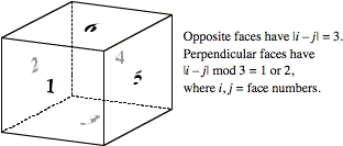
FIG. 9. Cyclic face numbering advantages.

It is important for a benchmark program to be concise and manageable, to minimize conversion effort and maintenance costs, yet represent the demands of a real computer application. These terse setup portions of the benchmark take only about 200 lines of a high-level computer language.

By using closed form expressions, the f_ij factors inherit the property that ∑_j f_ij ≈ 1, for all i, when correctly evaluated. Since each f_ij requires hundreds of operations to evaluate (including square roots, logarithms, and arctangents), this summation provides a sensitive independent test of the matrix setup. We choose a tolerance of 0.5 ´ 10^–8 for the ∑_j f_ij to deviate from unity, that is, an accuracy of 7 decimals. This requires somewhat more than “single-precision” arithmetic on most computers (7.4 decimals ideally, but fewer because of cumulative errors) but is comfortably within the “double-precision” range. This provides a level playing field for various arithmetic formats. It is usually advantageous to use the smallest number of bits or digits that satisfies the tolerance. This number will vary with problem size, but the user is free to meet the tolerance by adjusting precision as needed, throughout the task.

For ∑_j f_ij values within the tolerance limits but not numerically equal to unity, the f_ij values are normalized by the sum to force the sum to unity. This helps control minor cumulative rounding errors. Instead of normalizing the entire row of the matrix, we simply scale the right-hand side scalar and diagonal elements, trading n multiplications for two.

The area of patch i can be denoted a_i. Because the a_i are not all the same, f_ij ≠ f_ji in general (see Fig. 10).

FIG. 10. Asymmetric coupling.

This means that the radiosity matrix is nonsymmetric. However, in the process of trying to optimize the algorithm, we discovered that if the matrix rows are divided by a_i, the matrix becomes symmetric, as mentioned in Section 3.3. Symmetry reduces solution cost by roughly a factor of 2. Again, the scaling by a_i is applied to the diagonal and right-hand side, saving n² multiplications by 1/a_i of the other matrix elements. Cholesky factorization can be used for the matrix solution, for which there are well-tuned routines in many software libraries.

The second self-consistency test involves “residual” checks. For the linear system Ax = b, where A is an n by n matrix and x and b are vectors of n elements, the residual is defined as ||Ax – b||, where we choose a computationally easy norm, the maximum of the absolute values of the elements. To specify a tolerance, the residual is normalized by the norms of A and x, a quantity sometimes called the relative residual. We require that ||Ax – b|| / ||A|| ||x|| < 0.5 ´ 10^–8 for each of the x values computed by the benchmark (one x for each component of the radiation: red, green, and blue). Thus, the residual check is really three tests, all of which must pass. The residual check is performed after timing, since application software would generally eliminate such tests once program errors appeared to have been removed.

The choice of residual value stems from experience with software errors; because the algorithm is stable, errors committed during matrix solution quickly damp out and can be missed by less sensitive tests. We have found that the 0.5 ´ 10^–8 tolerance value detects such errors. It represents a middle ground between the low answer precision needed for applications such as scene rendering and the high precision needed for applications like quantum chemistry.

The user is encouraged to use whatever means work best to reduce the residual to the required tolerance. The problem is well posed. Partial pivoting would add O(n²) floating-point comparison operations and introduce a serial bottleneck into the factoring algorithm. Diagonal dominance can be easily proved from the fact that reflectivity is less than unity and the sum of off-diagonal elements in a row is unity. Hence, the matrix is symmetric and positive definite; we encourage the use of well-tuned Cholesky factorization library routines.

The second self-consistency check greatly improves the rules under which the benchmark is run. Some parallel computers might favor iterative methods, or solution methods of very different internal composition from that of the one supplied. The alternative method merely has to satisfy the 0.5 ´ 10^–8 tolerance for the full range of possible inputs, and it is then deemed a fair method to use.

For this reason, the range of possible inputs has been carefully bounded. The faces can range in dimension from 1 to 100 on an edge and from 0.001 to 0.999 in reflectivity. Some cases in these ranges will be difficult to solve by iterative methods. For example, consider the box shown in Fig. 11.

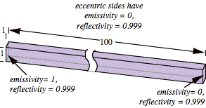
FIG. 11. Difficult iterative case.

Iterative methods must numerically accumulate enough terms of a slowly converging infinite series to account for the multiple low-loss reflections of radiation from the left face traveling down the box to the right. Just as

1 / (1 + x) ≈ 1 – x

favors the right-hand side for ease of computation when x is near 0,

1 / (1 + x) ≈ 1 – x + x² – x³ + … + x¹¹

will favor the “direct method” on the left if x is slightly larger than –1. Although multiple methods are permitted in the algorithm, we reserve the right to test using any input geometry within these bounds and to use the worst-case performance when there is variation depending on input data. In this manner, we constrain competing computers to use methods that are similar (that is, direct solvers), but not by artificial rules. The rules are instead driven by requirements for the output delivered to the user.

3.5. Figure of Merit

The notion of using operation counts or other “work” measures for computer performance evaluation has several drawbacks. It tends to reward inefficient methods that exercise the hardware, even if they get the result more slowly. The notion of what to consider an “operation” has not stood the test of time. In the 1950s and 1960s, multiplications dominated overall run time for compute-intensive problems, so complexity analysis considered only multiply and divide counts. By the 1970s, additions and multiplications had comparable cost and were often weighted equally. Now, memory references often take longer than the arithmetic, but are much harder to assess analytically for an abstract computer.

To date, the generally accepted practice has been to use execution time as the figure or merit, fixing the problem to be timed. This has disadvantages already described, but at least execution time is a physically measurable quantity.

Here, we make problem size the figure of merit (the larger the better), another measurable quantity not subject to dispute. The use of problem size can lead to slightly unconventional ranking of computers, as shown in Table I:

TABLE I

Differences in Figure of Merit

Computer A Computer B

1392 patches 1433 patches

2.75 billion operations (?) 2.99 billion operations (?)

51 s 59 s

53.9 MFLOPS (?) 50.7 MFLOPS (?)

By conventional measures, Computer A is ranked higher in performance since it performed more (estimated) MFLOPS. By the metric proposed here, Computer B is ranked higher because it ran a larger problem (more patches). Perhaps Computer A has difficulty applying its speed to a slightly larger run because it runs out of fast memory, exceeds a hardware vector length, etc. The effect will generally be only a slight difference from the MFLOPS-based ranking, except when the MFLOPS for a computer is a jagged function of the problem size. Computers A and B appear virtually identical, but the example is designed to illustrate how we remove any reliance on operation counts in assessing performance. Operation counts are subject to debate. Ours are estimated from the best-known serial algorithm and might be much lower than the operations actually performed by a parallel or vector computer.

Since supercomputer purchases are generally motivated by a desire to run larger problems (not achieve higher MFLOPS rates), the problem size makes a better figure of merit. This is the “grand challenge” esthetic. It contrasts, say, with the esthetic of maximizing conventional data processing throughput. The achievement of a 40,000-patch SLALOM run might be more significant than the achievement of a “teraflop” of nominal speed, since there would be at least a little assurance that the speed might be applicable to real problems.

3.6. Complete Task Measurement

The idea of a fixed-time benchmark solves the decades-old difficulty of including such parts of the benchmark execution as program loading, input, output, and other tasks with rather invariant time cost. With a fixed-sized problem, these components eventually dominate total execution time as vector or parallel methods are applied to the compute-intensive portions of the job (Amdahl’s 1967 argument against parallel architectures). Hence, previous benchmarks have solved the problem by including only the kernel in the timing, with an enormous loss of realism.

With a fixed time of about 1-min, the non-kernel part of the work should take just a few seconds, and can be included in the timing without distortion effects. For the radiosity problem described here, time should grow as

O(1) for program loading,

O(1) for reading problem geometry,

O(n²) for setting up the matrix,

O(n³) for solving the matrix, and

O(n) for storing the solution.

Traditional benchmarks time only the O(n³) part, or possibly both the O(n²) and the O(n³) parts. Here we time everything essential to the run other than the original writing and compiling of the program (which is presumably amortized over many runs and hence legitimate to neglect). Interestingly, the lower-exponent parts of the problem are the hardest to make run in parallel, so massively parallel architectures will reveal the same input/output challenges for SLALOM that they face in general applications.

3.7. Minimization of Human Effort Bias

To reduce the effect of variable human analytical skill in adapting a given program to a particular computer, we apply the same technique already mentioned in Section 3.3: a variety of best-effort versions are maintained in the library of possible starting points, for as many different architectures and languages as possible. New versions, motivated by the desire of a vendor to show high performance, are added to the library rather than kept proprietary. In this way, contributors must provide not just performance data but also their method for achieving that performance in software, so that others may build on their accomplishment.

4. SLALOM Profiling and Superlinear Speedup Effects

The preceding section gives SLALOM performance as a single number. We now consider a profile, or breakdown by task, of SLALOM performance. Much insight can be gained simply by examining three components of the total work: input/output, equation setup, and solution of the equations. Figure 12 shows typical variation in the profile with problem size. The figure illustrates the fallacy of MFLOPS as a performance metric. Functions such as input/output involve few floating-point operations, yet are an important component of the work. Similar problems would occur with MIPS, MOPS, etc.

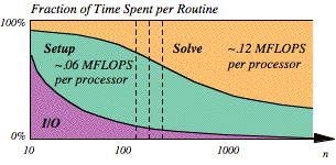
FIG. 12. Routine fraction vs. problem size.

If one relies on MFLOPS to measure speed, then superlinear speedup results when problem scaling causes more time to be spent in “faster” routines. Consider the matrix setup and matrix factoring parts of SLALOM. The setup will take order n² work and the factoring will take order n³ work. For small problems, setup might dominate the work, depending on the cost per matrix entry. The factoring approaches 100% of the work as n increases. Both steps can readily be done in parallel. In the fixed-time model, the fraction of the time spent on factoring increases with the number of processors. If the factoring proceeds at a higher speed than the setup (often the case), then each processor will run faster (more work per second) as the result of using more processors.

This reasoning is the theory of superlinear speedup by shifting algorithm profile. This form of superlinear speedup does not appear to have been previously described in the literature [4, 8, 10]. To test it experimentally, we used a version of SLALOM for the first-generation nCUBE computer. The speed in MFLOPS, as a function of P, was measured as shown in Table II:

TABLE II

Speedup on SLALOM

P Problem size, n MFLOPS Speedup

1 112 0.067 1.00

2 150 0.138 2.06

4 200 0.279 4.16

Even after extensive use of assembly language tuning, the problem setup ran at only 0.06 MFLOPS per processor, because of calls to intrinsic functions and irregular sequences of operations. The matrix solution, however, ran at 0.12 MFLOPS for large n. For the single-processor run, problem setup took 60% of the time, so the speed was close to 0.06 MFLOPS. On four processors, the larger n possible in a 1-min run causes factorization to take more of the time, so the speed per processor increased to about 0.07 MFLOPS. The effect would have been more dramatic except for the lack of parallelism in the input, output, and backsolving tasks. With further work, these will run in parallel and the superlinearity should approach about sixfold speedup on four processors. Figure 12 illustrates the effect described, with the vertical dashed lines representing the cases in Table II.

It is more accurate to note that the MFLOPS rates within each shaded region are not constant with n. Figure 13 shows this third dimension, using polynomial fits for experimental measurements on a SUN 4/370:

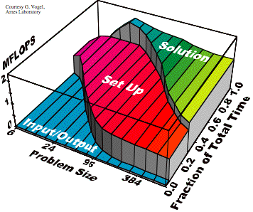
FIG. 13. Profile vs. n vs. MFLOPS rate.

The use of fixed-time performance models clearly affects the traditional notion of speedup. It has similar impact on the traditional definition of “efficiency.” The preceding examples show that efficiency can exceed unity, if one makes the naïve assumption that the uniprocessor speed is independent of the problem size. Profiling SLALOM and other fixed-time tasks is useful in understanding the reasons underlying the overall performance, but caution should be exercised in attempting to use profiling in conjunction with a conventional speed measure like MFLOPS.

5. BENCHMARK RESULTS

Table III gives some results of using the SLALOM benchmark on a wide range of computers. The computers are listed in order of decreasing problem size that they were able to solve. The list is a subset of the computers measured to date, selected to indicate the spectrum of SLALOM on computers available in the years 1990–1991. At least a dozen distinct architectural categories are represented, depending on one’s taxonomy. All times were close to 60 s, so the execution time is not given. Using the operation count of the best serial algorithm, one can estimate MFLOPS ranging from 2130 to 0.000646 for the first and last computers listed.

TABLE III

SLALOM Performance for Various Computers

Computer, environment Procs Patches Measurer Date

Cray Y-MP8, 167 MHz 8 5120 J. Brooks (v) 9/21/90

Fortran+tuned LAPACK Cray Research

nCUBE 2, 20 MHz 1024 3736 J. Gustafson 2/8/91

Fortran+assembler Ames Lab

Cray-2S/8, 244 MHz 8 2443 S. Elbert 9/8/90

Fortran+directives Ames Lab

Intel iPSC/860, 40 MHz, 64 2167 T. Dunigan 1/7/91

Fortran+assembler BLAS ORNL

MasPar MP-1, 12.5 MHz 16384 2047 J. Brown (v) 11/20/90

C with plural variables (mpl) MasPar

Alliant FX/2800 14 1736 J. Perry (v) 1/24/91

Fortran (-Ogc, KAI Lib's) Alliant

nCUBE 2, 20 MHz 64 1623 J. Gustafson 4/8/91

Fortran+assembler Ames Lab

IBM 3090-200VF 1 1549 J. Shearer (v) 1/9/91

Fortran+ESSL calls, opt(3) IBM

Silicon Graphics 4D/380S 8 1352 O. Schreiber (v) 4/2/91

33 MHz, Fortran+block Solver Silicon Graphics

IBM RS/6000 540, 30 MHz 1 1304 J. Shearer (v) 1/8/91

Fortran+ESSL calls, XLF V2 , -O IBM

FPS M511EA, 33 MHz 1 1197 B. Whitney (v) 1/24/91

Fortran+LAPACK calls FPS Computing

IBM RS/6000 520, 20 MHz 1 1091 J. Shearer (v) 1/9/91

Fortran+ESSL calls, XLF V2 , -O IBM

IBM RS/6000 320, 20 MHz 1 895 S. Elbert 1/30/91

Fortran+block Solver (-O -lblas) Ames Lab

SKYbolt, 40 MHz i860/i960 1 831 C. Boozer (v) 1/9/91

C+assembler dot product SKY Computers

SKYstation, 40 MHz i860/i960 1 793 C. Boozer (v) 1/29/91

C (-O sched vec UNROLL) SKY Computers

Silicon Graphics 4D/35 1 717 O. Schreiber (v) 1/29/91

37 MHz, Fortran, (-O2 -mp) Silicon Graphics

FPS-500 (33 MHz MIPS + vec.) 1 619 P. Hinker 11/12/90

Fortran (FPS F77 4.3,-Oc vec) LANL

DECStation 5000, 25 MHz, 1 534 S. Elbert 1/30/91

Fortran+block Solver (-O2) Ames Lab

Silicon Graphics 4D/25, 20 MHz 1 507 S. Elbert 1/30/91

Fortran+block Solver (f77 -O2) Ames Lab

DECStation 5000, 1 432 D. Rover 1/31/91

25 MHz, Pascal (-O2) Ames Lab

SUN 4/370, 25 MHz, 1 419 M. Carter 10/8/90

C (ucc -O4 -dalign etc.) Ames Lab

DECStation 3100, 16.7 MHz 1 418 S. Elbert 1/30/91

Fortran+block Solver (-O2) Ames Lab

Sil. Graphics 4D/20, 12.5 MHz 1 401 S. Elbert 1/30/91

Fortran+block Solver (f77 -O2) Ames Lab

Myrias SPS-2, 68020, 16.7 MHz 64 399 J. Roche (v) 6/21/90

Fortran (mpfc -Ofr) Myrias

DECStation 2100, 12.5 MHz 1 377 S. Elbert 1/30/91

Fortran+block Solver (-O2) Ames Lab

Motorola MVME181, 20 MHz 1 289 R. Blech 10/17/90

Fortran, (OASYS F77 1.8.5) NASA

Sequent Symmetry 33 MHz 1 253 M. Carter 1/3/91

C (cc -O -fpa) Ames Lab

VAXStation 3520 1 181 M. Carter 1/24/91

C (cc -O) Ames Lab

Cogent XTM (T800 Transputer) 1 149 C. Vollum (v) 6/11/90

Fortran 77 (-O -u) Cogent Research

Toshiba 1000, 6 MHz 8088 1 12 P. Hinker 11/14/90

C (Turbo C, with reg/jump option) LANL

NOTES

A “(v)” after the name of the person who made the measurement indicates a vendor. Vendors frequently have access to compilers, libraries, and other tools that make their performance higher than that achievable by a customer.

The CRAY Y-MP runs failed the old SetUp3 tolerance of 0.5 ´ 10^–10, but passed with a tolerance of 0.5 ´ 10^–8; special logarithm and arctangent functions were used with only 11-decimal precision for higher speed. We will enforce the current tolerance uniformly in future reports.

The CRAY 2/8 above is a unique eight-processor computer at Lawrence Livermore National Laboratory. The CRAY 2 figures are low compared to those of the CRAY Y-MP because blocking methods were not used; future runs will use matrix–matrix multiply as the kernel, as was done for the Y-MP.

MFLOPS assume O(n³) cost for matrix factoring and are likely to be inaccurate (too large) for problems that use block methods with O(n^2.8) Strassen multiplication or better.

6. CONCLUSIONS

The fixed-time concept is a simple one. To be practical, it requires an application that scales smoothly over a wide range. If the selected application can exploit distributed memory parallelism, it can be used to obtain meaningful performance evaluation over the wide range of ensemble sizes characteristic of distributed memory computers. We have tried to meet these goals, and other goals of a more general nature, in designing the SLALOM benchmark.

SLALOM illustrates a new source of non-spurious superlinear speedup. Specifically, speed per processor is not constant as problems scale; it changes with fraction of time spent in routines of different algorithmic complexity. This superlinear result is perhaps best regarded as a symptom of the fallacy of using MFLOPS or other simplistic speed measures, and not as an exceptionally effective use of parallel processors.

We view SLALOM as a step toward providing a level playing field for advanced architectures. We are committed to maintaining the scientific integrity of this benchmark and look forward to measuring and publishing even more wide-ranging SLALOM numbers in the future. The response since SLALOM was announced in November of 1990 has been quite positive, and dozens of researchers have contributed to our performance database. We hope that the scalability of the benchmark will allow it to last several decades without a fundamental change. It may be the first benchmark with such longevity and will permit the tracking of technology trends over a wide baseline.

ACKNOWLEDGMENTS

We thank everyone who has participated in this effort. In particular, analysts at Alliant, Cogent, Cray, IBM, Intel, MasPar, and Myrias have contributed suggestions, ideas, and versions of the SLALOM program. Much of the work was performed at the Scalable Computing Laboratory at Ames Laboratory/Center for Physical and Computational Mathematics.

REFERENCES

1. Benner, R. E., Montry, G. R., and Gustafson, J. L. A structural analysis algorithm for massively parallel computers. In Carey, G. F. (Ed.). Parallel Supercomputing: Methods, Algorithms, and Applications, Wiley Series in Parallel Computing, Wiley, New York, 1989.

2 Curnow and Wichmann, A synthetic benchmark. Computer Journal, (Feb 1976).

3. Dongarra, J. J., Performance of various computers using standard linear equations software in a Fortran environment. Tech. Memorandum 23, Argonne National Laboratory, Feb. 2, 1988.

4. Faber, V., Lubeck, O., and White, A., Superlinear speedup of an efficient sequential algorithm is not possible. Parallel Computing, 3 (1986), 259–260.

5. Goral, C. M., Torrance, K. E, Greenberg, D. P., and Battaile, B., Modeling the interaction of light between diffuse surfaces. Comput. Graphics 18, 3 (July 1984).

6. Gustafson, J. L., Reevaluating Amdahl’s law. Comm. of the ACM, 31, 5 (May 1988).

7. Gustafson, J. L., Montry, G. R., and Benner, R. E., Development of parallel methods for a 1024-processor hypercube. SIAM Journal on Scientific and Statistical Computing, 9, 4, (July 1988).

8. Helmbold. D. P., and McDowell, C. E., Modeling speedup(n) greater than n. 1989 Proc. International Conference on Parallel Processing, 1989, Volume III, pp. 219–225.

9. McMahon, F. M., The Livermore Fortran kernels: a computer test of numerical performance range. Tech. Rep. UCRL-55745, Lawrence Livermore National Laboratory, University of California, Oct. 1986.

10. Parkinson, D., Parallel efficiency can be greater than unity. Parallel Comput., 3 (1986), pp. 261–262.

11. Pointer, L., PERFECT: Performance evaluation for cost-effective transformations, Report 2. CSRD Report 964, Mar. 1990.

12. Randell, B. (Ed.). The Origins of Digital Computers: Selected Papers. Springer-Verlag, New York/Berlin, 1975, 2nd ed., pp. 84, 138, 227, 229, 283, 306.

13. Seitz, C. L., The cosmic cube. Comm. of the ACM 28 (1985), 22–23.

14. Smith, J. E., Characterizing performance with a single number. Comm. of the ACM 31, 10 (Oct. 1988), 1202–1206.

15. SPEC. SPEC Benchmark Suite Release 1.0. Oct. 1989.

16. Sun, X.-H., and Ni, L., Another view on parallel speedup. Proc. Supercomputing ’90. IEEE Computer Society, Silver Spring, MD, 1990, pp. 324–333.

17. Weicker, R. P., Dhrystone: A synthetic systems programming benchmark. Comm. of the ACM 27, 10 (Oct. 1984).

18. Worley, P. H., The effect of time constraints on scaled speedup. Rep. ORNL/TM-11031, Oak Ridge National Laboratory, Jan. 1989.

________________________________________________________________________

JOHN GUSTAFSON received the B.S. degree in applied mathematics from Caltech in 1977 and the M.S. and the Ph.D. from Iowa State University in 1981 and 1982, respectively. He was Product Development Manager and Senior Staff Scientist at Floating Point Systems from 1982 to 1986, Staff Scientist at nCUBE from 1986 to 1987, and a member of the Technical Staff at Sandia National Laboratories from 1987 to 1989. His work on the 1024-processor hypercube at Sandia, with colleagues Gary Montry and Robert Benner, won the inaugural Gordon Bell award in 1988. Since 1989, he has led research efforts in massively parallel computing at the Ames Laboratory. Dr. Gustafson is a Subject Area Editor for Performance Evaluation for the Journal of Parallel and Distributed Computing. His interests include computational physics and chemistry, novel performance metrics, and parallel algorithms. He is a member of SIAM.

DIANE ROVER received the B.S. degree in computer science in 1984, the M.S. degree in computer engineering in 1986, and the Ph.D. degree in computer engineering in 1989, all from Iowa State University. From 1985 to 1988, she was awarded an IBM Graduate Fellowship. In 1986, Dr. Rover was an intern with McDonnell Douglas Corp., and in 1987, with the IBM Thomas J. Watson Research Center. Since 1983, she has been a Technical Education Consultant for IBM. She is currently a postdoctoral researcher in the Scalable Computing Laboratory at the Ames Laboratory. Her research interests include parallel processing, computer architecture, performance evaluation, instrumentation, and performance visualization. Dr. Rover is a member of the IEEE Computer Society, the Association for Computing Machinery, Sigma Xi, and the Society of Women Engineers.

STEPHEN ELBERT received the B.S. degree in chemistry from Iowa State University in 1968 and the Ph.D. in theoretical chemistry from the University of Washington in 1973. He was a postdoctoral fellow at the University of Bonn from 1973 to 1975 and at Iowa State from 1975 to 1977. Since 1977, he has been a research scientist on the staff of the Ames Laboratory. His research interests include large scale ab initio quantum chemistry calculations to determine the reaction surfaces of small molecules, with particular emphasis on the efficiency of the algorithms involved. He is a member of Sigma Xi.

MICHAEL CARTER received the B.S and M.S. degrees in electrical engineering from Oklahoma State University in 1987 and 1989, respectively, and is a Ph.D. candidate in the Department of Electrical Engineering and Computer Engineering at Iowa State University. His interests include image synthesis, parallel algorithms, and computer architecture. Mr. Carter is a member of the ACM, IEEE Computer Society, Phi Kappa Phi, and Tau Beta Pi. He is currently a research assistant at the Scalable Computing Laboratory at the Ames Laboratory.