Abstract. We have developed a fast parallel version of an existing
synthetic aperture radar (SAR) simulation program, SRIM. On a 1024-processor NCUBE hypercube, it
runs an order of magnitude faster than on a CRAY X-MP or CRAY Y-MP processor.
This speed advantage is coupled with an order of magnitude advantage in machine
acquisition cost. SRIM
is a somewhat large (30,000 lines of Fortran 77) program designed for
uniprocessors; its restructuring for a hypercube provides new lessons in the
task of altering older serial programs to run well on modern parallel
architectures. We describe the techniques used for parallelization, and the
performance obtained. Several novel approaches to problems of task
distribution, data distribution, and direct output were required. These
techniques increase performance and appear to have general applicability for
massive parallelism. We describe the hierarchy necessary to dynamically manage
(i.e., load balance) a
large ensemble. The ensemble is used in a heterogeneous manner, with different programs on
different parts of the hypercube. The heterogeneous approach takes advantage of
the independent instruction streams possible on MIMD machines.
Keywords. Algorithms, hypercubes, load balancing,
parallel processing, program conversion, radar simulation, ray tracing, SAR.
*This work was
performed at Sandia National Laboratories, operated for the U. S. Department of
Energy under contract number DE-AC04-76DP00789, and was partially supported by
the Applied Mathematical Sciences Program of the U. S. Department of Energy's
Office of Energy Research.
1.
INTRODUCTION
We
are developing parallel methods, algorithms, and applications for massively
parallel computers. This includes the development of production-quality
software, such as the radar simulation program SRIM, for execution on massively parallel
systems. Here, massive parallelism refers to general-purpose Multiple-Instruction, Multiple-Data
(MIMD) systems with more than 1000 autonomous floating-point processors (such
as the NCUBE/ten used in this study) in contrast to Single-Instruction, Multiple-Data
(SIMD) systems of one-bit processors, such as the Goodyear MPP or Connection
Machine.
Previous work at Sandia has shown that regular PDE-type problems can achieve near-perfect speedup on 1024 processors, even when all I/O is taken into account. The work described in [9] made use of static load balancing, regular problem domains, and replication of the executable program on every node. This is the canonical use [8] of a hypercube multicomputer [6, 10, 11, 17], and we observed speeds 1.6 to 4 times that of a conventional vector supercomputer on our 1024-processor ensemble.
We
now extend our efforts to problems with dynamic load balancing requirements,
global data sets, and third-party application programs too large and complex to
replicate on every processor. The performance advantage of the ensemble over
conventional supercomputers appears to increase with the size and irregularity of the
program; this observation is in agreement with other studies [7]. On a radar
simulation program, SRIM,
we are currently reaching speeds 7.9 times that of the CRAY X-MP (8.5 nsec
clock cycle, using the SSD, single processor) and 6.8 times that of the CRAY
Y-MP. This advantage results primarily from the non-vector nature of the
application and the relative high speed of the NCUBE on scalar memory
references and branching. Since either CRAY is 12–20 times more expensive than
the NCUBE/ten, we can estimate that our parallel version is at least 15 to 25
times more cost-effective than a CRAY version using all four or eight of its
processors.
The
SRIM application is
one of importance to Sandia’s mission. It permits a user to preview the
appearance of an object detected with synthetic aperture radar (SAR), by
varying properties of the view (azimuth, elevation, ray firing resolution) and
of the radar (wavelength, transfer function, polarization, clutter levels,
system noise levels, output sampling). SRIM is based on ray-tracing and SAR modeling
principles, some of which are similar to those used in optical scene
generation. Hundreds of hours are consumed on supercomputers each year by the SRIM application.
Successful restructuring of SRIM required that parallel application
development draw upon new and ongoing research in four major areas:
- heterogeneous programming
- program decomposition
- dynamic, asynchronous load balancing
- parallel graphics and other input/output
These
four areas are the focus of this paper. The resulting performance of parallel SRIM represents major performance and cost
advantages of the massively parallel approach over conventional vector
supercomputers on a real application.
In
§ 2, we examine background issues. These include the traditional approach
to ray tracing, characteristics of the third-party simulation package, SRIM [1], salient features of our 1024-processor
ensemble, and how those features fit the task of radar simulation. We then
explain in § 3 the strategy for decomposing the program—both spatially and
temporally—with particular attention to distributed memory and control. The
performance is then given in
§ 4, and compared to that of representative minicomputers and
vector supercomputers.
2. BACKGROUND DISCUSSION
2.1 TRADITIONAL RAY TRACING AND
PARALLELISM
The
ray-tracing technique has its origin at the Mathematical Applications Group,
Inc. (MAGI) in the mid-1960s [12, 13]. Ray tracing was first regarded as a
realistic but intractable method of rendering images, since the computations
could take hours to days per scene using the computers of that era. As
computers became faster, use of the ray tracing technique increased.
In
optical ray tracing, a light source and a set of objects are stored as
geometrical descriptions. Rays from the viewer are generated on a grid or
randomly. The rays are tested for intersection against the entire set of
objects as shown schematically in Figure 1. A “bounce” is recorded for each ray
that experiences at least one intersection. That is, the first intersection is
found by sorting and treated as a generator of another ray. The set of records
associated with these ray bounces is known as the ray history. The process repeats until the ray leaves
the scene or the number of bounces exceeds a predetermined threshold. The
effect (line-of-sight returns) of the original ray on the viewer can then be
established.
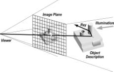
Figure 1. Traditional Ray Tracing
(Optical)
The ray firing events are operationally independent, so the problem appears to decompose so completely that no interprocessor communication is necessary. It is a common fallacy that putting such an application on a parallel processor is a trivial undertaking. Although the rays are independent, the object descriptions are not. Also, the work needed for each ray is uneven and the resulting work imbalance cannot be predicted without actually performing the computation.
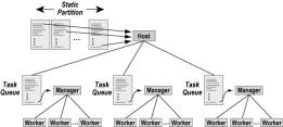
Therefore,
some form of dynamic, asynchronous load balancing is needed to use multiple
processors efficiently. A common approach, inadequate for our 1024-processor
ensemble, is the master-slave model,
with the host delegating tasks from a queue to processors that report in as
idle. Figure 2 illustrates this scheme. On a hypercube, a logarithmic-height
spanning tree provides the required star-shaped topology. This is handled by
the hypercube operating system and need not be visible to the programmer.
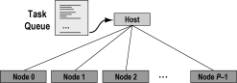
Figure 2. Master-Slave Load Balancer on a Hypercube
Simple
master-slave schemes do not scale with the number of slave processors. Suppose,
as in our hypercube, that the host uses at least two milliseconds to receive
even the shortest message from a node. If all 1024 nodes send just a two-byte
message indicating their work status to the host, the host must spend a total
of two seconds just receiving all the messages. If the average node task takes
less than 2 sec, the host will be overwhelmed by its management responsibilities
and the nodes will often be in an idle state waiting for the host for new
assignments. A much better method is described in § 3.3 below.
An
entirely different approach is to divide space rather than the set of fired rays, which
potentially removes the need for every processor to be able to access the
entire object database. This approach creates severe load imbalance near the
light sources and high interprocessor communication cost; see [15].
2.2 PROBLEM SCALING
The algorithmic cost of a ray-tracing algorithm depends primarily on:
- The number of rays
fired
- The maximum allowed number of bounces
- The number of objects
in the scene
The increase in
computational effort and the amount of ray history data is approximately linear
in the number of rays fired. However, memory requirements are unaffected by the number
of rays, because ray history data resides in either an SSD scratch file on the
CRAY or interprocessor messages on the hypercube.
The maximum allowed number of bounces b can affect computational effort, since every bounce requires testing for intersection with every object in the scene. In some optical ray tracing models, rays can split as the result of reflections/refractions, causing work to increase geometrically with maximum bounces. Here, we increase work only arithmetically. As with the number of rays fired, varying b has little effect on storage requirements. Therefore, it is possible, in principle, to compare elapsed times on one processor and a thousand processors for a fixed-size problem [9], since scaling the problem does not result in additional storage. These scaling properties contrast with those of the applications presented in [9], in which increasing ensemble size leads naturally to an increase in the number of degrees of freedom in the problem.
2.3 THE SRIM RADAR SIMULATOR
The
SRIM program has about
30,000 lines (about 150 subroutines) of Fortran 77 source text. The two most
time-consuming phases are GIFT (18,000 lines), and RADSIM (12,000 lines). GIFT reads in files from disk describing the scene geometry,
and viewpoint information from the user via a console, and then computes “ray
histories,” the geometrical paths traced by each ray fired from the emanation
plane. It has its roots in the original MAGI program [4], and uses
combinatorial solid geometry to represent objects as Boolean operations on
various geometric solids. In contrast to many other ray tracing programs that
have been demonstrated on parallel machines, GIFT supports many primitive geometrical
element types:
Box 4
to 8 Vertex Polyhedron
Sphere Elliptic
Hyperboloid
General
Ellipsoid Hyperbolic
Cylinder
Truncated
General Cone Right
Circular Cylinder
Truncated
Elliptical Cone Rectangular
Parallelepiped
Half-Space Right
Elliptic Cylinder
Truncated
Right Cone Arbitrary
Polyhedron
Circular
Torus Parabolic
Cylinder
Elliptical
Paraboloid Right-Angle
Wedge
Arbitrary
Wedge Elliptical
Torus
This
large number of object types is a major reason for the large size of the serial
GIFT executable
program.
To
reduce the need to compare rays with every object in the database, GIFT makes use of nested bounding boxes that
greatly reduce the computational complexity of the search for intersections.
For the price of additional objects in the database, the cost of the comparison
is reducible from linear to logarithmic complexity in the number of objects.
A
subset of GIFT
converts a text file describing the geometries to a binary file that is then
faster to process. However, it is common to convert a text file to binary once
for every several hundred simulated images, much as one might compile a program
once for every several hundred production runs. Therefore, we have not included
the conversion routine in either the parallelization effort (§ 3) or
performance measurement (§ 4).
The
ray histories generated by serial GIFT are also stored on disk (SSD on the CRAY version). RADSIM, a separately loaded program, then uses
this ray history file to simulate the effect on a viewing plane of radar
following those paths (see Figure 3.) By separating the simulation into these
two parts, the user can experiment with different radar properties without
recomputing the paths taken by the rays.
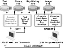
Figure 3. Serial SRIM Flowchart
Unlike
optical ray tracing, every object intersection visible from the viewing plane contributes to
the image, and the contributions add as complex numbers instead of simply as
real intensities. That is, interference between waves is a significant effect.
Also unlike optical ray tracing, the ray-traced image must be convolved with
the original radar signal (usually by FFT methods). Another difference from
optical ray tracing is that dozens of bounces might be needed to obtain an
accurate image. While optical ray tracing algorithms might reduce computation
by setting a maximum of three to ten bounces, synthetic aperture radar often
undergoes over 30 bounces without significant attenuation.
Perhaps
the most important qualitative difference between SAR and optical imagery is
that the x-axis does
not represent viewing azimuth in SAR images. Instead, it represents the length
of the path from the radar source to the target. Thus, the SAR image may bear
little resemblance to the optical image. This is one reason users of SAR (as
well as systems for automatic target recognition) must be trained to recognize
objects; they cannot rely on simple correspondence with the optical appearance
of targets. As a result, large databases of SAR images are needed for every
object of interest, which poses a daunting computational task.
The
RADSIM approach is
described in [1]. Other methods for predicting radar signatures are described
in [5]. The so-called dipole approximation method, or method of moments, takes into account the fact that
conductors struck by electromagnetic radiation become radiation sources
themselves, creating a large set of fully-coupled equations. Radiosity
methods [3] for
predicting optical images also lead to fully coupled equations. Although the
dipole and radiosity methods are in principle more accurate than ray tracing,
the cost of solving the resulting dense matrix restricts the method of moments
to relatively coarse descriptions of scenes and objects.
2.3 THE 1024-PROCESSOR ENSEMBLE AND SRIM ISSUES
The
NCUBE/ten is the largest Multiple-Instruction Multiple-Data (MIMD) machine
currently available commercially. The use of processors specifically designed
as hypercube nodes allows ensembles of up to 1024 processors to fit in a single
cabinet. Each node consists of the processor chip and six 1-Mbit memory chips
(512 Kbytes plus error correction code) [14]. Each processor chip contains a
complete processor, 11 bidirectional communications channels, and an
error-correcting memory interface. The processor architecture resembles that of
a VAX-11/780 with floating-point accelerator, and can independently run a complete
problem of practical size. Both 32-bit and 64-bit IEEE floating-point
arithmetic are integral to the chip and to the instruction set; currently, SRIM primarily requires 32-bit arithmetic.
Since
there is no vector hardware in the NCUBE, there is no penalty for irregular,
scalar computations. This is appropriate for the SRIM application, since vector operations play
only a minor role in its present set of algorithms. Also, much of the time in SRIM is spent doing scalar memory references
and testing for the intersection of lines with quadratic surfaces, which
involves scalar branch, square root, and divide operations. Since each NCUBE
processor takes only 0.27 microsecond for a scalar memory reference, 1
microsecond for a branch, and 5 microseconds for a square root or divide, the
composite throughput of the ensemble on those operations is 50 to 550 times
that of a single CRAY X-MP processor (8.5 nanosecond clock).
All
memory is distributed in our present hypercube environment. Information is
shared between processors by explicit communications across channels (as
opposed to the shared memory approach of storing data in a common memory). This
is both the greatest strength and the greatest weakness of ensemble computers:
The multiple independent paths to memory provide very high bandwidth at low
cost, but global data structures must either be duplicated on every node or
explicitly distributed and managed.
Specifically,
there is no way a single geometry description can be placed where it can be
transparently accessed by every processor. Each processor has 512 Kbytes of
memory, of which about 465 Kbytes is available to the user. However, 465 Kbytes
is not sufficient for both the GIFT executable program (110 Kbytes) and its database, for the most
complicated models of interest to our simulation efforts. It is also
insufficient to hold both the RADSIM executable program (51 Kbytes) and a high-resolution output
image. (The memory restrictions will be eased considerably on the next
generation of hypercube hardware.) Our current parallel implementation supports
a database of about 1100 primitive solids and radar images of 200 by 200 pixels
(each pixel created by an 8-byte complex number). Two areas of current research
are distribution of the object database and the radar image, which would remove
the above limitations at the cost of more interprocessor communication.
The
hypercube provides adequate external bandwidth to avoid I/O bottlenecks on the SRIM application (up to 9 Mbytes/sec per I/O
device, including software cost [2]). It is also worthy of note that for the
1024-processor ensemble, the lower 512 processors communicate to the higher 512
processors with a composite bandwidth of over 500 Mbytes/sec. This means that
we can divide the program into two parts, each running on half the ensemble,
and have fast internal communication from one part to the other.
The
host may dispense various programs to different subsets of the ensemble,
decomposing the job into parts much like the data is decomposed into
subdomains. Duplication of the entire program on every node, like duplication
of data structures on every node, is an impractical luxury when the program and
data consume many megabytes of storage. This use of heterogeneous
programming reduces
program memory requirements and eliminates scratch file I/O (§ 3.1). With
respect to program memory, heterogeneous programming is to parallel ensembles
what overlay
capability is to serial processors; heterogeneous programming is spatial,
whereas overlays are temporal.
One
more aspect of the system that is exploited is the scalability of distributed
memory computers, which makes possible personal, four-processor versions of the
hypercube hosted by a PC-AT compatible. We strive to maintain scalability
because the performance of personal systems on SRIM is sufficient for low-resolution studies
and geometry file setup and validation. Also, since both host and node are
binary compatible with their counterparts in the 1024-processor system, much of
the purely mechanical effort of program conversion was done on personal
systems.
3. PARALLELIZATION
STRATEGY
To
date we have used four general techniques to make SRIM
efficient on a parallel ensemble: heterogeneous ensemble use (reducing disk
I/O), program decomposition (reducing program storage), hierarchical task
assignment (balancing workloads), and parallel graphics (reducing output time).
3.1 HETEROGENEOUS
ENSEMBLE USE
As
remarked above, traced rays are independent in optical ray tracing. In the SRIM radar simulator, the task of tracing any one
ray is broken further into the tasks of computing the ray history (GIFT) and computing the effect of that ray on
the image (RADSIM). In
optical ray tracing, the latter task is simple, but in radar simulation it can
be as compute-intensive as the former.
The
serial version completes all ray histories before it begins to compute the
effect of the rays on the image. We extend the parallelism within these tasks
by pipelining them (Figure 4); results from nodes running GIFT are fed directly to the nodes simultaneously
running RADSIM, with
buffering to reduce the number of messages and hence communication startup
time. We divide the parallel ensemble in half to approximately balance the load
between program parts; depending on the maximum number of bounces and the
number of objects, processing times for GIFT are within a factor of two of processing
times for RADSIM. Why
is this heterogeneous approach better than running GIFT on all nodes, then RADSIM on all nodes, keeping the cube
homogeneous in function?
First,
it eliminates generation of the ray history file, thereby reducing time for
external I/O. Although the ray history file in principle allows experiments
with different radar types, practical experience shows that it is always
treated as a scratch file. The human interaction, or the preparation of
databases of views of an object, invariably involves modifications to the viewing
angle or object
geometry instead of just
the radar properties. Hence, only unused functionality is lost, and we avoid
both the time and the storage needs associated with large (~200 Mbyte)
temporary disk files. (Applying this technique to the CRAY would have only a
small effect, since scratch file I/O on the SSD takes only 3% of the total
elapsed time.)
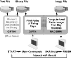
Figure 4. Parallel SRIM Flowchart
Secondly,
it doubles the grain size per processor. By using half the ensemble in each phase, each
node has twice as many tasks to do. This approximately halves the percent of
time spent in parallel overhead (e.g. graphics, disk I/O) in each program part. Furthermore, by having
both program parts in the computer simultaneously, we eliminate the serial cost
of reloading each program part.
3.2. PROGRAM
DECOMPOSITION
As
shown in Figure 3 above, the original serial version of SRIM exists in two load modules that each
divide into two parts. Since every additional byte of executable program is one
less byte for geometric descriptions, we divide SRIM into phases to minimize the size of the
program parts. Some of these phases are concurrent (pipelined), while others
remain sequential.
First,
we place I/O management functions, including all user interaction, on the host.
Most of these functions, except error reporting, occur in the topmost levels of
the call trees of both GIFT and RADSIM.
They include all queries to the user regarding what geometry file to use, the
viewing angle, whether to trace the ground plane, etc., as well as opening,
reading, writing, and closing of disk files. Much of the program (83500 bytes
of executable program) was eventually moved to the host, leaving the
computationally intensive routines on the much faster hypercube nodes, and
freeing up their memory space for more detailed geometry description. Both GIFT and RADSIM host drivers were combined into a single
program. This was the most time-consuming part of the conversion of SRIM to run in parallel. To illustrate the
host-node program decomposition, Figure 5 shows the original call tree for RADSIM. (The call tree for GIFT is too large to show here.
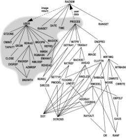
Figure 5. Call Tree for Radar Image Generation
The
parts of the program run on the host are shown in the shaded region in Figure
5. The others run on each RADSIM hypercube node. The dashed lines show messages between hypercube
nodes and the host program. One such path is the communication of the computed
radar image from RADSIM
to subroutine USER on
the host. The other is the PROCES subroutine, which has been divided into host and node routines
that communicate program input by messages. Routines RDHEAD and EMANAT in the host portion are also needed by
the node; these were replicated in the node program to eliminate the calling
tree connection. The GIFT program contained many subroutines that had to be replicated on
both host and node in a rather arduous process of separating host and node functionality.
Error
reporting can happen at any level in the program, a common practice in Fortran.
To remove the need for computationally-intensive subroutines to communicate
with the user, errors are reported by sending an error number with a special
message type to the host, which waits for such messages after execution of the GIFT and RADSIM programs begins.
Next,
the conversion of text to binary geometry files was broken into a separate
program from GIFT. We
use only the host to create the binary geometry file. The conversion program, CVT, uses many subroutines of GIFT, so this decomposition only reduces the
size of the executable GIFT program from 131 Kbytes to 110 Kbytes.
Similarly,
the convolution routines in RADSIM are treated separately. Much of the user interaction involves
unconvolved images and, unlike the ray history file, the unconvolved image
files are both relatively small and repeatedly used thereafter. This reduces
the size of the RADSIM
executable program, allowing more space for the final image data in each node
running RADSIM.
One
option in SRIM is to
produce an optical image instead of a radar image. Since this option is mainly
for previewing the object, ray tracing is restricted to one bounce for greater
speed. Although optical and the radar processing are similar and use many of
the same routines, only the executable program associated with one option needs
to be loaded into processors. The user sets the desired option via host queries
before the hypercube is loaded, so breaking the program into separate versions
for optical and radar processing further reduces the size of the node
executable program.
Finally, we wish to display the radar images quickly on a graphics monitor. This means writing a program for the I/O processors on the NCUBE RT Graphics System [14]. These I/O processors are identical to the hypercube processors except they have only 128 Kbytes of local memory. Although library routines for moving images to the graphics monitor are available, we find that we get a 10- to 30-fold increase in performance [2] by crafting our own using specific information about the parallel graphics hardware.
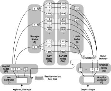
Figure 6 summarizes the division of the hypercube into subsets performing different functions. There are currently eight different functions in our parallel version of SRIM:
· Host program
· Host I/O node program (the VORTEX operating system; no user program)
· Manager node program (currently part of GIFT)
· GIFT node program
· Image node program (currently part of RADSIM)
· RADSIM node program
· Graphics node program
· Graphics controller program (loaded by user, supplied by the vendor)
We
have not fully optimized the layout shown in Figure 6. For example, it may be
advantageous to reverse the mapping of the GIFT Manager program and RADSIM Image program to the nodes, to place the RADSIM nodes one communication step closer [2, 15] to the
graphics nodes. Also, a significant performance increase (as much as 15%)
should be possible by driving disk I/O through the parallel disk system instead
of the host disk, in the same manner that graphics data is now handled by the
parallel graphics system. Successful use of parallel disk I/O requires that we
complete software which renders the parallel disk system transparent to the
casual user, so that portability is maintained between the 1024-processor
system and the four-processor development systems.