PURPOSE-BASED BENCHMARKS
J. Gustafson
SUN MICROSYSTEMS, INC., USA
Summary
We define an approach to
benchmarking, Purpose-Based Benchmarks, which explicitly and comprehensively
measures the ability of a computing system to reach a goal of human interest. This
contrasts with the traditional approach of defining a benchmark as a task to be
timed, or as the rate at which some activity is performed. Purpose-Based
Benchmarks are more difficult to create than traditional benchmarks, but have a
profound advantage that makes them well worth the trouble: They provide a
well-defined quantitative measure of the productivity of a computer
system.
1 Introduction
Purpose-Based Benchmarks provide a means for assessing
computer productivity. The focus of this paper is the motivation and methods
for designing such benchmarks. Elsewhere in this volume, [Faulk et al. 2004] make use of this
benchmark approach as a core component of productivity analysis, and focus on
human factors analysis and the measurement of software life cycle costs.
1.1 BENCHMARK DESIGN GOALS
Benchmarks are tests of
computer systems that nominally serve two main purposes [Kahan 1997]:
1) to help potential users of systems estimate the performance
of a system on their workload, prior to purchase, and
2) to help system designers optimize their designs before
finalizing their choices.
Implicit in both of these is the idea that the
benchmark is low-cost or quick, compared to running a full customer workload
(or actually building a system.) However, some historical benchmarks have
ignored this common-sense aspect of benchmarking and have created tests that
cost many man-months of effort and over a hundred thousand dollars to run.
Ideally, benchmarks should maximize the amount of guidance they provide for the
least possible effort.
The most common aspect of a computer that benchmarks
test is “speed.” However, speed on a computer is not a well-defined measure.
Computer “speed” lacks the properties we demand of metrics in physics, like
meters per second or degrees Kelvin [Snelling 1993]. The reason is that
computer speed is “work” divided by time and computer “work” is not well defined.
The standard workaround for this is to attempt to define a fixed task as the
work, and consider only the reciprocal of the execution time as the figure of
merit that we call “speed.” Another common approach is to treat quantities like
“transactions” or “floating-point operations” or “logical inferences” as atomic
units of work that can be used as the numerator in the speed definition. However,
this approach fails because the quantities being counted vary greatly in
individual complexity and difficulty, and hence cannot be used as scientific
units.
1.2 THE BENCHMARK-WORKLOAD GAP
Every benchmark sets up an adversarial
relationship if the benchmark designer and the benchmark user are different
parties. Even if a test is used within a company to assess a proposed design,
the engineers are highly motivated to show that their choices yield favorable
results. However, the primary tension of benchmarking is between marketing
departments and potential customers. As soon as a benchmark becomes widely
used, the feature subset that it exercises becomes overvalued. This sets up a
dynamic in which the vendor can reduce its costs by neglecting parts of workloads
that are not tested by the benchmark, even though they might be quite important
to the customer.
One response to this is to create a large suite
of tests, in the hope that somehow every aspect of a workload is covered.
However, this raises the cost of running the benchmark, and might not succeed
in covering the total workload. SPEC and PERFECT Club are examples of efforts
at achieving general workload coverage through the amassing of program examples
that seem qualitatively different in some respect. It takes only slightly
longer for vendors to tune their offerings in such a way that they perform well
on these suites but not on applications in general.
The message here is one for the benchmark
designer: Assume people will exploit any difference between the benchmark and
the actual workload, because there will always be motivation to use a benchmark
not as a scientific tool but as a persuasion tool. Put another way, the
consumer of benchmark information thinks: “This only tests a subset of the
machine properties, but I can probably assume that the untested things are
similar in performance.” The benchmark measurer thinks: “This only tests a
subset of the machine properties, so I can sacrifice the performance of
everything that isn’t tested.” Both situations exploit the benchmark-workload
gap.
The following examples show the types of things
the author has watched go wrong in benchmarking because of the adversarial tension:
Example: A benchmark allows reporting of the best performance achieved, not the median
or mean. Therefore, the benchmark measurer runs it twenty times and manages to
find and report the rare case that performs 30% better than it does on average.
Example: A benchmark requires that 64-bit floating-point data be used throughout,
but only checks that the answer is correct to a few decimals. Therefore, the
benchmark measurer uses quick approximations for all of the intrinsic functions
like sin(x), ex, and log(x), each valid to only four decimal places, saving 20% of the run time.
Example: A benchmark states a large set of activities to perform, but only asks
that some of the results be printed or displayed. Therefore, the benchmark
measurer uses a compiler that tacitly eliminates any code that does not affect
the output, effectively “running” large portions of the benchmark in no time at
all.
Example: A small (kernel) benchmark, like many benchmarks, only measures the execution
time but not the time to create the executable code. Therefore, the benchmark
measurer uses a compiler that requires four days to exhaustively optimize the
kernel operation, and the program then runs in 11 seconds instead of 16
seconds. The benchmark measurer is further able to boast that no assembly language
or hand tuning was needed to achieve this 45% speed improvement.
Example: A benchmark measures both processor time and the time for I/O from disk,
and thereby captures the time for scratch I/O, the time to read in the problem
description, and the time to write out the final answer. But it doesn’t time
the ten minutes it takes to load the program into an 8000-processor system with
a poorly-designed operating system… so what’s claimed as a 14-minute run really
took 24 minutes total.
Example: A benchmark requires that only a single processor be tested. Therefore,
the benchmark measurer disables the processors in an eight-processor architecture
while leaving their caches and memory controllers active, allowing the entire
benchmark to fit into the local cache and run in half the time it would for any
configuration that a person would actually elect to use.
Example: A benchmark measures a standalone system, since the statistical effect of
other users who share the system seems difficult to incorporate into the
benchmark rules. So, a person who buys a system based on the standalone
benchmark is alarmed to discover that the system takes two minutes to roll one
task out and another task in, making the system far less productive in actual
use than the benchmark predicted. The system designers had no motive to make
context switching fast since they knew it was not measured by the benchmark.
Example: A benchmark based on an application program always uses the same input
data, even though the application program is capable of running a large range
of possible inputs. Therefore, after the benchmark has been in common use for
about three years, the benchmark measurers have learned to make that specific
data set run fast even though doing so has reduced the average speed for the
full range of possible input.
Specific names of institutions and people who
have employed these techniques are not given in these examples, because the
intent is not to assign blame. The intent is to illustrate how traditional
benchmark design inevitably leads to such distortions.
As the benchmark designers discover each of
these unintended consequences of their imprecise rules, they add rules to stop
people from abusing the test in that particular way. This is the approach of
the SPEC consortium, for example. Enforcement of such rules is difficult or
impossible in some cases.
A better approach is to define the benchmark
in a way that aligns with real computer use so closely, that “cheating” is no
longer cheating. Any method found to run a real workload faster or better is inherently a
legitimate design improvement and not a cheat. Where there is no gap between
workload and benchmark, no cheating is possible. Section 2 will describe this
approach in detail.
1.3 PRINCIPLES FOR REPORTING
RESULTS
The High-Performance Computing (HPC) community
is surprisingly lax in applying standards of scientific reporting. When a
scientific paper is published announcing an experimental result, the authors
expect to be held accountable for the validity of their claims. Yet, many HPC
benchmarks are reported with anonymous, undated database entries that are not
reproducible by third parties. If a clever technique is invented that allows a
higher score, the submitters are in many cases allowed to keep their technique
secret so that it becomes a competitive advantage; consumers of the data are
misled that one system is superior, when the superiority actually lies in the
cleverness of the programmer.
In general, we should demand
the following of any benchmark report:
1) The date the test was made
2) Who ran the test and how they may be contacted
3) The precise description of what the test conditions
were, sufficient that someone else could reproduce the results within
statistical errors
4) The software that was used, and an explanation for any
modifications made to what is generally available as the definition of the
benchmark
5) An accounting of cost, including the published
price of the system and any software that was used in the run.
6) An accounting, even if approximate, of the amount of
time spent porting the benchmark to the target system.
7) Admission of any financial connections between vendor
and the reporter; was the system a gift? Do they work directly for the vendor
or for a contractor of the vendor?
8) The range of results observed for the test, not just the
most flattering results. The reporters should reveal the statistical
distribution, even if there are very few data points.
The last several requirements go beyond the
reporting needed for scientific papers. They must, because of the direct
marketing implications of the reports. Scientific papers usually don’t imply
purchasing advice, the way benchmark reports do. The bar for benchmark reporting
must be even higher than it is for scientific publishing.
1.4 A MINIMAL REPRESENTATIVE SET
Benchmark suites tend to grow beyond the size
they need to be, for the simple reason that users refuse to believe that their
requirements are represented unless they see a part of the suite that uses
their same vocabulary and seems superficially to resemble their own workload.
Thus, a program for finding the flow of air
around a moving automobile might solve equations very similar to those of a
weather prediction model, and use the same number of variables and operations,
but the automotive engineer would refuse to accept a weather benchmark as
predictive. Thus, benchmark components proliferate until they become almost unmanageable.
When the underlying demands of a workload are
analyzed into machine-specific aspects like cache misses, fine-grain
parallelism, or use of integer versus floating point operations, applications
look even more similar than one might think. For example, even “compute-intensive”
problems rarely contain more than 5% floating-point operations in their instruction
traces, and 2% is typical. [IBM 1986] Our intuitive prejudice that each
technical application area deserves its own operation mix may not withstand scrutiny.
The more profound differences that need to be
representative are things like problem size. In circuit design, for
example, 95% of the work might be small jobs that run in a few minutes and
easily fit into a 32-bit address space; but the other 5% involve full-chip
simulations that require 64-bit addressing and a very different set of system
features to run well. Yet, both are in the “EDA market.”
To use a transportation analogy, the difference
in performance of two cars in commuting a distance of 20 miles is not apt to be
very great, and probably does not depend that heavily on the city for which the
commute is measured if the cities are about the same size. However, imagine the
time to commute into a town of 2000 people being used to predict the time to
commute into a town of two million people. It’s patently absurd, so we know better than
to lump those measures together into a single category called “commuting workload.”
Getting the problem size right is perhaps the
most important single thing to match in using a benchmark to predict a real
workload. This is especially important in the HPC arena. Yet, it is usually the
first thing to be thrown out by benchmark designers, since they want a small
problem that is easy to test and fits a wide range of system sizes.
1.5 BENCHMARK EVOLUTION
1.5.1 Activity-Based Benchmarks. For decades, the benchmarks
used for technical computing have been activity-based. That is, they select certain
operation types as typical of application codes, then describe an example of
those activities with which to exercise any particular computer. When accuracy
is considered at all, it is not reported as a dimension of the performance.
Current examples include
STREAM: Measure the time for simple vector operations
on vectors of meaningless data, of a length chosen to exercise the main addressable
memory. Assume answers are valid. The activity measure is “bytes per second.”
Confusion persists regarding whether distributed memory computers are allowed
to confine their byte moves to local memory [McCalpin].
GUPS: Measure
the rate at which a system can add 1 to random locations in the addressable memory
of the computing system. The activity measure is “updates per second.”
Confusion persists regarding whether distributed memory computers are allowed
to confine their updates to local memory, and the level of correctness
checking. While the latest official definition is the RandomAccess benchmark,
this definition is quite different from TableToy, the original benchmark that
measures GUPS.
LINPACK: Measure the time to use a
1980s-style linear equation solver on a dense nonsymmetric matrix populated
with random data. Measure answer validity, but discard this information in
reporting and comparing results. The activity measure is “floating-point
operations per second.” [Dongarra]
The inadequacy of these activity-based tests
for tasks (1) and (2) above is obvious. Neither the activities nor the metrics
applied to them have anything to do with actual user workloads. Their only
merit is that they are very easy to run. Scientists and engineers understand
that these are simply activity rates, but many take it on faith that activity
rates correlate with the ability of the computer to help them solve problems.
The LINPACK benchmark, which survives mainly as
a “Top 500” ranking contest, uses rules that place the measurement of activity
above the measurement of accomplishing a purpose. We now have methods for solving
linear equations, based on Strassen multiplication, that run in less time and give results that are more
accurate. However, the maintainers of the LINPACK rankings explicitly forbid
Strassen methods, because Strassen methods invalidate the floating-point
operation count. That is, the activity measure uses the older Gaussian
elimination method to determine the operation count. Strassen methods require
fewer operations to get the answer. Getting better answers faster via a better
algorithm is a violation of LINPACK rules.
1.5.2 Application
Suite Approach. In an effort to make benchmarks more representative than these small
kernel operations, benchmark designers have collected existing application
programs and packaged them as benchmarks [SPEC, Pointer 1990]. This packaging generally
includes:
1) Insertion of timer calls so that the program times its
own execution. (“Execution” does not include the time to compile the program or
load it into a system; sometimes it does not even include the time to load
initial data from mass storage or write the answer to mass storage.)
2) An effort to restrict the source text to the subset of
the language likely to compile correctly on a wide range of commercial systems.
3) A set of rules limiting what can be done to obtain
flattering timings.
4) A collection of results from other systems to use for
comparison.
5) A specific data set on which to run the application,
usually selected to be small enough to fit on the smallest systems of interest
at the time the benchmark is declared.
There is usually little attention to answer
validity [Kahan 1997]. Sometimes an example output is provided, and the person
performing the run must examine the output and decide if the answers are “close
enough” to the example output to be acceptable.
1.5.3 Accommodation
of New Architectures. As parallel computers such as the Thinking Machines CM-1, Intel iPSC, and
nCUBE 10 became available as commercial offerings, users found existing benchmark
approaches inadequate for prediction and comparison with traditional architectures.
Users and designers alike found themselves retreating to raw machine
specifications like peak FLOPS and total memory, since those metrics were
determinable and applied as systems scaled from uniprocessors to thousands of
processors.
In making the “application suite” benchmark approach
apply to parallel systems, one is immediately faced with the question of how to
scale the benchmark without losing the experimental control over what is being
compared. Obviously, larger systems are for running larger problems; however,
application suites invariably fix the size of the problem and have no way to
compare the work done by a large system with the smaller amount of work done by
a small system
The NAS Parallel Benchmarks are typical in this
respect; every time they need a different benchmark size, they must produce a
new set of sample output to use as the correctness test [Bailey and Barton,
1991]. This means the NAS Parallel Benchmarks are not, in fact, scalable. They
are simply different benchmarks available in different sizes. The new
architectures demanded scalable benchmarks where the “work” could be fairly defined
and measured.
1.5.4 Attempts
at Algorithm Independence. In the early 1990s, technical benchmarks were introduced that showed
alternatives to activity-based benchmarking, and allowed true scaling of the
problem.
SLALOM [Gustafson et al., 1991] had a kernel similar to
LINPACK, but fixed the execution time at one minute and used the amount of
detail in the answer (the number of patches in the domain decomposition for a
radiosity computation) as the figure of merit. It was language-independent,
allowed any algorithm to be used, and included the time for reading the problem
from mass storage, setting up the system of equations, and writing the answer
to mass storage. It was the first truly scalable scientific benchmark, since
the problem scaled up to the amount of computing power available and was
self-validating.
SLALOM had a fatal flaw: The test geometry was
symmetric, and researchers eventually found ways to exploit that symmetry to
reduce the work needed compared to the general case. The rules had failed to
specify that the method had to work on a general geometry. The definition of
answer validity (answer self-consistency to 8 decimal digits) was better than
previous scientific benchmarks, but still arbitrary and not derived from real
application goals. The lesson we learned from this was the need to subject
algorithm-independent benchmarks to extensive preliminary review by innovative
people before releasing the benchmark definitions for general use.
The HINT benchmark [Gustafson and Snell, 1995]
finally established a rigorous figure of merit: The accuracy of a numerical
integration. HINT scales to any size without needing comparison against a pre-computed
answer set. By defining the purpose instead of the activity (“Minimize the
difference between the upper and lower bound of the area under a curve”), a
level playing field was finally created for fair comparison of vastly different
computer systems. The person using the benchmark can use any numerical
precision, floating point or integer type. Version 1.0 of HINT is still in use;
it has remained valid through six cycles of Moore’s law and shows no sign of
needing redefinition. Its only shortcoming as a benchmark is that the problem
it solves is of little human interest.
1.5.5 Grand
Challenges, ASCI, and HPCS. During the 1990s, the discrepancy between HPC benchmarks and federal
program goals became too great to ignore. The “Grand Challenge” program for
supercomputing was so lacking in precise goal measures that it experienced a
loss of congressional support for funding [Weingarten 1993, Gustafson 1995].
The ASCI program set a goal of a “100 teraflops computer by 2004,” repeating
the assumption that peak floating-point activity rate, by itself, closely
predicts the ability to produce useful physical simulations. The emphasis on
floating-point speed created a generation of large computing systems that had
high arithmetic speed but were unreliable, hard to use, and hard to administer.
Recognizing this, in the early 2000s DARPA developed
a program, High Productivity Computing Systems (HPCS), to re-emphasize all
those aspects of computer systems that had been neglected in the various giant
computer projects of the previous decade. DARPA recognized that existing
benchmarks were incapable of holistic productivity measurement, and made the
development of new and better metrics a key goal of the HPCS program.
The next step in benchmark evolution became
clear: Can we create benchmarks that have rigorous definitions of progress
toward a goal of real human interest, so that they can measure the actual productivity of
computer systems?
2 Purpose-Based
Benchmarks
2.1 DEFINITION
A purpose-based benchmark (PBB) states an objective of
direct interest to humans. For example, “Accurately predict the weather in the
U.S. for the next three days” is a starting point for a more precise description
of something to be done, and a complete PBB supplies both English and
mathematical definitions of the task and the figure of merit. It does not tell how to accomplish the
task with a computer, leaving the benchmark measurer free to use any means
available. Whatever technique is used, however, must be supplied in such a way
that any other benchmark measurer could use that technique if they wished, or
else the benchmark results are not considered valid and publishable.
For those who wish to test a computer system
without testing the program development effort, a PBB provides a set of reference
implementations. This is simply to allow people to focus on the execution performance
if they wish to ignore program development effort. It is very important that
the productivity of a novel architecture not be measured starting from an
inappropriate reference implementation. If a system demands a starting point
that is not similar to one of the reference implementations, then the time to
develop an appropriate starting point must be measured separately as program
development effort.
The hardest part of designing a PBB is to find
a quantitative measure of how well a system achieves its purpose. The
floating-point arithmetic used in scientific calculations yields different
answers depending on the algorithm, the compiler, and the actual precision in
the hardware (including registers with guard bits). Given this, how can we
fairly compare completely different algorithms and architectures?
In the weather example, we can compare against
physical reality. Where this is impractical, we seek tasks for which the
quality of the answer can be calculated rigorously by the computer itself. In
both cases, methods such as Interval Arithmetic can play a key role by measuring
the uncertainty in the answer [Hansen and Walster, 2004]. This is in contrast,
say, to measuring problem quality by the number of grid points; adding grid
points does not always increase physical accuracy in simulations. We are
accumulating problems for which both the physics and the solution method are
sufficiently rigorous that the answer can be bounded or self-checked, because
that provides a quantitative measure of how well a program meets its purpose.
Note that the PBB approach can measure
productivity using legacy codes and does not require a completely new program
to be written, for those problems where a quantitative measure of answer
quality can be rigorously defined. The primary departure from the conventional
use of legacy codes as benchmarks is that one must measure aspects other than
just the execution time. For example, a PBB statement for electronic design
might be to design an n-bit adder and test it, with the purpose of making the circuit fast, small,
and provably correct. Users of electronic design codes do not mainly write
their own software, but obtain it from independent software vendors. Hence, a
PBB for electronic design could compare existing software packages to see which
one results in the best productivity for the complete task of designing the
adder.
Making data-specific tuning is obviously
impossible in the case of predicting the weather. Note that there is no need to
state what kind of arithmetic is used (like 64-bit or 32-bit floating point),
since any arithmetic that accomplishes the purpose is legitimate. Benchmark
measurers are encouraged to be economical in the activity performed by the
computer, so doing more operations per second is no longer a goal in itself. In
fact, aiming for more operations per second might lower the score on a PBB
because it leads one to use less sophisticated algorithms [Gustafson 1994].
2.2 ACCEPTABILITY FUNCTIONS
The concept of Utility is defined in game theory
[Luce and Raiffa, 1957]. It is a scalar ranging from –¥ to +¥ that
attempts to quantify the value humans place on outcomes so that different
strategies can be compared. We use a related concept here, that of Acceptability. The Acceptability
Function of
an aspect of a computer system is the fraction of users (in a particular
field) who deem the system acceptable. Unlike Utility, Acceptability ranges from 0 to 1.
Acceptability Functions were first proposed as a way to give quantitative
meaning to the vague goals of the U.S. “Grand Challenge” computing program [Gustafson
1994].
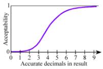
Acceptability Functions
quantify the nonlinearity of the utility of many computer features. For
example, if one computes π, having only one digit of accuracy in the result is
unacceptable for most applications; six digits might suffice for most
applications, but 60 digits of π is seldom worth ten times as much to a user as six
digits! The Acceptability climbs from near zero (unacceptable) for single-digit
accuracy to near unity (completely acceptable) for six or seven digits of accuracy.
Figure 1. Acceptability Function Example
Here are some qualities of
computer systems that are amenable to Acceptability function analysis:
• Reliability (fraction of runs that complete satisfactorily)
• Availability (fraction of the time that the system can be used
for the problem)
• Precision (relative or absolute accuracy of the results)
• Time to port or develop the application
• Time to boot the system from a cold start
• Time to load the system with the application
• Time to execute the application
• Acquisition cost of the system
• Operational cost per hour of the system (or cost of each run),
including all administrative costs
• Space required (footprint or volume) for physical system
• Power required and heat
dissipated
For all of these aspects, each user has numbers
X and Y for which they will say
“Worse than X is unacceptable. Better than Y and we don’t care.” Instead of guessing about those
numbers, or letting them be implied and unstated, we can declare the
assumptions for each application area and let users in that area debate their
correctness. If a user says “The cheaper your system, the better,” he has
implied a linear utility for the system cost and a lack of concern, say, with
reliability.
There’s an old saying in marketing: “Fast,
cheap, and good… pick any two.” We can actually give this idea serious
treatment by requiring that ∏Ai be at least, say, 0.9 for all the Acceptability
functions Ai. If computer procurements were stated in such terms, there would be much
better communication of requirements between users and system designers.
The aforementioned problems with repeatability,
time to compile, reliability, time to load, and so on, can all be incorporated
into an Acceptability Product. The Acceptability Product is the product of the Acceptability
Functions. If a particular aspect is more important, then it can be given
greater weight simply by making its function steeper or altering where it
changes from 0 to 1.
What traditional benchmarking does not take
into account is that this nonlinearity applies to execution time… and that the Acceptability
curve varies widely from one application area to another. In fact, one might
define a technical computing market as a collection of customers with similar
Acceptability curves as well as similar workloads.
High-energy physicists have a culture of planning
large-scale experiments and waiting months for the results. In using supercomputers to
test the viability of theories (like quantum chromodynamics, or searching for
rare events in acquired data), they show similar patience and are willing to
consider computer jobs requiring months to complete. If given more computing
power, they would almost certainly escalate the problem being attempted instead
of doing the same task in less time. If they don’t, other scientists with more
patience will make the discoveries first.
The 24-hour weather forecast must be completed
and submitted in three hours, in practice. Forecasters have found that the
effort to update or extrapolate stale input data becomes so arduous at some
point that a 24-hour forecast would never finish or would be too inaccurate to
be useful.
In military applications, like using a computer
to determine whether a tank is that of a friend or a foe, any time longer than
a few seconds might be fatal. On the other hand, there is little difference
between taking 0.2 second and 0.1 second to compute, since human response time
is then greater than the computing time.
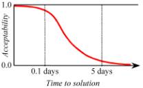
The following is a possible Acceptability
function of execution time, for a particular application area:
Figure 2. Time Acceptability Example
This leads directly to the question of whether
a benchmark has to last the same amount of time as the actual workload, in
order to be representative and have predictive value. If the only way to
predict the performance on a ten-month-long physics run is to test the machine
for ten months, then the benchmark itself is prohibitively expensive and
becomes useless in such situations. Whereas business applications quickly reach
steady-state behavior that permits accurate sampling, many technical
applications progress through phases that make highly varying demands on the
system hardware and software. It is not simply a matter of “warming the cache”
in some cases. Therefore, any simplification of HPC workloads must be validated
scientifically to show that the reduced problem produces results that correlate
with the actual workload.
2.3 EXAMPLE: PBB FOR STRUCTURAL ANALYSIS
(TRUSS OPTIMIZATION)
We now bring all these measurement principles
to bear in a benchmark designed to capture the workload of engineers who use
computers to assist in structural analysis [Mullen and Muhanna, 1999]. Typical
problems in Mechanical Computer-Aided Engineering (MCAE) are
• Find the stresses and strains in a design to see if it meets
requirements.
• Optimize a design for a particular feature, like low weight or
low cost or high efficiency.
• Find out if the design has resonant modes that could cause
failure when shaken (buildings, bridges, engines, etc.)
This motivates the purpose of the benchmark problem.
We also pay attention to the other aspects of this segment that determine the
other Acceptability functions. Answer validity is of extreme importance,
because failures may lead to loss of life or many millions of dollars in
damage. Hence, the cost acceptability function is related to the amount of
damage (and losses from lawsuits) that the computer can prevent. Also, note
that in the design of a large structure, the position of the parts probably
must be specified to a precision comparable to other sources of errors in the
part manufacturing and assembly. For example, 0.1 millimeter is probably overkill
in a large structure, and 60 millimeters is probably out of tolerance. Finally,
we note that mechanical engineers are accustomed to waiting several hours for
an answer, even overnight, which is still not such a long time that it delays
the construction of a proposed mechanical object. This takes into account the
trial-and-error time needed, not just a single static solution for a proposed
design.
This is the basis for the “Truss” benchmark, which
we now define. It is clearly far simpler and more specific than the gamut of
mechanical engineering tasks, but it appears representative of much of the
workload.
2.3.1 English
Statement of Purpose. Given a set of three attachment points on a vertical surface and a point
away from the surface that must bear a load, find a pin-connected steel truss
structure that uses as little steel as possible to bear the given load. The
structure must be rigid, but not overdetermined. Cables and struts vary in
thickness based on the forces they must bear, including their own weight and
the weight of the connecting joints. Start with no added joints, which defines
the unoptimized weight w0:
Figure 3. Initial Truss Problem, No Extra Joints
The attachment points vary from
problem to problem. The system does not know the attachment point coordinates
until the run begins. The point in space where the load is located, the amount of the load, and
the strength of the steel (tensile and compressional failure) are similarly
subject to variation so that the benchmark cannot be “wired” to a particular
data set.
2.3.2 Mathematical Problem Formulation. The benchmark is not intended
to test the structural analysis expertise of a programmer; the complete
definition supplies the explanation that a “domain expert” in MCAE might supply
a programmer to enable the Truss program to be created.
The force equilibrium requirement gives rise to
a set of linear equations. The Truss PBB uses a “free body” approach. It does
not require finite element analysis. However, it produces equations that have
very similar structure to those used everywhere in structural analysis
(positive definite, symmetric, sparse).
The net force on every joint must be zero, or
else the truss would accelerate instead of being at equilibrium. (The vertical
surface, being fixed, will supply a countering force to anything applied to
it.) The weight of each member produces an additional downward force that is
split evenly between its endpoints.
These principals, plus formulas for the
strengths of struts and cables, complete the information needed to create a
working Truss optimization program.
2.3.3 Parallelization
Strategies. There
is enough work in Truss to keep even a petascale computer quite busy for hours,
because the set of possible truss topologies grows very rapidly with the number
of joints.
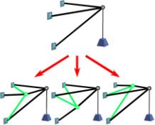
Figure 4. Parallel Topology Optimization
The outermost level of
parallelization is the topology generation. Even a small number of joints
generates billions of designs to test. The next level is the optimization of
any given topology, each of which can be spread over a large set of process
threads. The innermost level of parallelism is that of solving the sparse and
relatively small set of linear equations. This solving is iterative because
once the thickness of each truss or cable is determined from the applied
forces, the resulting weights must be used to recompute the load until the
solution converges. Interval arithmetic can be used to exclude certain
topologies or joint positions, and this exclusion needs to be communicated to
all processors so that future searching can be “pruned” [Hansen and Walster,
2004]. Load balancing and constant global communication create a representative
challenge for large-scale scientific computers.
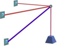
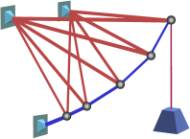
Figure 5 shows a truss that
was optimized by an early form of this PBB. The blue lines represent struts (compressive
load), and the red lines represent cables.
Figure 5. Optimized Truss Structure
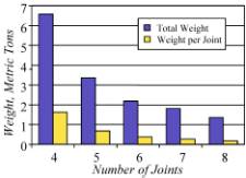
The weight reduction possible by adding
complexity is dramatic, lest anyone think that all this computing is
unnecessary. Figure 6 shows the drop in weight of the truss as joints are
added, using a topology similar to that shown in Figure 5.
Figure 6. Weight Reduction with Complexity
2.3.4 Acceptability Functions. The most important Ai are the ones that show
Acceptability as a function of the reduction in weight, the accuracy of the
answer, the time to perform the run, and the cost of the computer run. Many
others could be included, but let’s start with these.
The initial guess is to connect single beams
and cables from the attachment points to the load point. This is the heaviest
solution and easy to compute, so it defines the starting value. If we are
unable to reduce the weight, the Acceptability is zero. If we could by some
incredibly ingenious method reduce the weight to nothing (a sort of gossamer
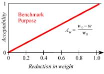
structure), then Acceptability would be one. The purpose that defines this purpose-based
benchmark thus becomes one of the Acceptability functions. Acceptability = (Reduction
of weight) divided by (Initial weight). This is a simple linear function of the
weight w
and the unoptimized weight w0:
Aw = (w0–
w)/w0:
Figure 7. Truss Benchmark Purpose
Acceptability Function
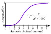
We can estimate the
Acceptability function for the accuracy of the answer. This function and the
ones that follow are purely for purposes of illustration, and the function is
an invented one that “looks right”; it must be replaced by one based on actual
studies of user requirements. For now, it serves as a number the computer can
calculate at the end of a benchmark run, using higher-quality (and slower)
arithmetic than was used during the run:
Figure 8. Accuracy Acceptability
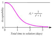
The time to perform the run
captures the patience typical of practitioners in this application area, which
is often dictated by the time required for the entire task. The actual construction
of a truss might require a few days to a few weeks, for example, so few
engineers would care about the difference between an instantaneous answer and
one that required, say, 15 minutes of computation. It is typical for structural
analysis programs to be adjusted in complexity to the point where a job started
at the end of the business day is finished by the beginning of the next
business day… about 15 hours. A run of less than 7 hours might be well accepted
(since it allows two runs per business day), but acceptance might drop to less
than 0.5 if a run takes an entire day. The following curve was constructed to
fit these estimates.
Figure 9. Acceptability of Solution Time
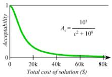
The cost of the run similarly
yields a decreasing Acceptability function. At first, the cost would appear to
be tied simply to the cost of the steel that is saved, which is probably only a
few thousand dollars. However, a characteristic of the structural analysis
segment is that the computation insures against a design failure that could
cost lives or result in catastrophic destruction of property. No one would
consider insuring a truss structure that had been designed without a quantitative
analysis regarding its strength and safety, because failure could cost millions
of dollars in lawsuits. The reasoning is similar to that used by actuaries to
determine the cost of liability insurance.
It is conceivable that some small fraction of
designers would be willing to spend over $50,000 to certify that a structure
meets all safety requirements while optimizing some aspect of the design. At
the other extreme, it may be petty to reduce the cost of the computer run
below, say, 0.1% of the cost of actually building the structure. Here is an
example of a possible Cost acceptability function:
Fig. 10. Acceptability of Cost
There are other Acceptability
functions that could be put into the Net Acceptability product, such as reliability
(fraction of runs that complete successfully), but we stop with these four for
now: A = AwAaAtAc.
This is a radical departure from the typical
way that cost and time are incorporated into benchmark reporting. Many
productivity measures use ratios to cost or ratios to time. This approach makes
more sense for traditional business computing, where cost and time are accurately
regarded as linearly disadvantageous. Taking twice as long or costing twice as
much is clearly half as productive for a given amount of output. This is much
less the case for high-end, technical computing.
2.3.5 Result Reporting and Verification. The Truss benchmark produces
an output that would be sufficient for an engineer to create the structure: the
list of joints, their position in space, the members that connect to them,
whether the members are cables or struts, and the length and cross-section of
each member. Since the input requirements have a random component to prevent
“cheating” on the benchmark, it is not immediately obvious how to verify that
the output is valid.
In addition to the output information listed
above, the benchmark requires that a list of forces impinging on each joint be
printed, and the sum of those forces. This makes clear whether the linear system was actually
solved, since the total force on every joint should be zero. The list of forces
is not so large that a human cannot scan it for validity, and of course, the
computer can easily compute the maximum deviation from zero of the list of net
joint forces as a single-value test of validity. We envision that the numerical
verification of the answer will use containment set methods that go well beyond
the arithmetic used to obtain the answer, and will be considered part of the
execution. These tests are in development at present.
2.4 OBJECTIONS TO THE PBB
APPROACH
The PBB approach was first presented to audiences in late 2002. Some of the
common reactions and responses follow.
You shouldn’t reduce
performance to a single number. It’s clearly a multidimensional quantity.
Yes, but if you don’t define a way to reduce it to a single number, someone
else will. Their summation probably will not be the one you envisioned. Therefore,
I strongly recommend that any benchmark present the multidimensional data and try to specify the single
figure of merit that best correlates with the way users would coalesce all
those values. Ultimately, people will reduce any collection of aspects to a
single number that determines whether they are willing to pay the price for the
system. The Acceptability Functions communicate what the assumed importance is
of each aspect of the system, but anyone can take the component measures and
apply their own set of Acceptability Functions to the same metrics. See [Smith
1988] for an in-depth discussion of the single-number reporting issue.
Since
the PBB rules are so loose, doesn’t that make it easy to cheat?
On the contrary, it makes cheating impossible by defining it away. Cheating
is possible only when there is a difference between user goals and what is actually
measured. In the ten years that HINT has been available, not a single method of
cheating has been found; this is for the reason stated. Imagine that someone
finds a way to “cheat” by predicting the weather more accurately with less
effort. How could that possibly be considered cheating? If some discrepancy is found between the user goals
and what the PBB measures, then the PBB is simply redefined to eliminate the
discrepancy.
You
have to be a real domain expert to use one of these things.
Not if we do our job right. While we need a domain expert to construct the
benchmark (and supply Acceptability criteria), understanding a PBB description
shouldn’t require a specialized degree in mechanical engineering or finance or
meteorology to understand. Both the purpose and the explanation of how to solve
the problem should be accessible to the educated public. The Truss benchmark,
for example, requires only high school physics to program once we provide the
rules for the strength of the cables and struts. Most of these problems require
a one-page lesson in the specific math and physics they require, but if they
require more than that, we probably have an unusable PBB and should redesign
it.
Doesn’t this just measure
the cleverness of the programmers instead of the system? What will happen if
someone comes up with a very clever way to solve the problem?
Whatever clever method is used, it must be shared with everyone as part of
the reporting of the benchmark. Others can then choose to use the technique or
not. Furthermore, since PBBs can (and should) take into account the development
cost, the use of clever programmers or extensive tuning effort will show up as
reduced Acceptability in the development cost aspect.
I don’t see how to make
my workload purpose-based.
The PBB approach
doesn’t work universally; at least it doesn’t yet. An example of a workload
that is difficult to make purpose-based is: “Run a simulation showing two galaxies
colliding.” Checking the simulations against actual experiment could take a
long time indeed. There is no attempt to establish the accuracy of the answer,
since the value of the computation is the qualitative insight it provides into
an astrophysical phenomenon. While we acknowledge the importance of programs
for which the output is judged in a non-numerical way, we do not currently have
a benchmark approach that encompasses them.
Why multiply the
Acceptability Functions together? Wouldn’t a weighted sum be better?
A
weighted sum makes sense for many “productivity” definitions, such as each
stage in a software life cycle, but “acceptability” has different implications
as an English word. The reason for using products is that one unacceptable parameter means the entire system is
unacceptable. That’s
easier to do with products than with weighted sums. Imagine a system that is
affordable, fast, and easy to program, but has just one problem: It never gets
the right answer. Should that failure be thrown into a weighted sum as just one
more thing to consider, or should it be given multiplicative “veto power” over
the single-number rating? There may be aspect pairs that represent tradeoffs,
where poorness in one aspect is compensated by excellence in another, and then
a weighted sum would be the right model. The Acceptability Product is similar
to what one sees in formal procurements for computer systems. The Acceptability
of the system is the logical AND of all the requirements being met, and not
expressed as tradeoffs.
I
have a computer program that solves a very interesting problem; can we make it
into a Purpose-Based Benchmark?
Many
people have presented the author with programs from their area of interest and
suggested that they be used to define a PBB. The usual obstacle is that there
is no quantitative definition of how well the program achieves its purpose, and
the person has no idea how to compare two completely different methods of
solving the problem that take the same amount of time but get different
answers. Once that’s done, the rest of the task of converting it to a PBB is
straightforward.
What you’re proposing is too difficult.
If what you
want to measure is Productivity, it’s difficult to see how it can be made simpler.
2.5 FUTURE WORK
One lesson from history is that benchmark definitions are
difficult to change once they are widely disseminated. Hence, we are doing very
careful internal testing of the PBBs before including them as part of a published
paper. We are testing the Truss PBB with college programming classes right now.
We will create versions in various languages and with various parallelization
paradigms (message passing, global address space, OpenMP) to use as starting
points for those who wish to test just the execution characteristics of a
system. Once these have had sufficient testing, we will disseminate them
through the Internet and traditional computing journals. While the temptation
was great to include an early version of a code definition of Truss in an
Appendix, this would almost certainly result in that becoming the community
definition of the benchmark prematurely.
A second PBB that involves radiation transport is nearly
complete in its English and mathematical definition. An I/O-intensive PBB based
on satellite image collection, comparison, and archiving is under review by
experts. A weather/climate PBB consists almost entirely of defining the quality
of a prediction, and we expect to use existing public-domain weather models as
reference implementations instead of attempting to develop our own. We are well
along in the creation of a biological PBB based on the purpose of using
computers to find the shapes and properties of proteins.
For each PBB, we are finding domain experts to review the
benchmarks and verify that the workloads are representative and
give initial feedback on the Acceptability Functions. Eventually, the
Acceptability Functions should be determined by statistical survey of users in
particular application areas, and updated periodically. A third-party
institution such as IDC might be ideal for this task.
SUMMARY
The
Purpose-Based Benchmark approach represents the latest in an evolving series of
improvements to the way computer systems are evaluated. The key is the expression
of an explicit purpose for a computation, and a way to measure progress toward
that goal as a scalar value. They are particularly well suited to technical
computing because they solve the long-standing problem of comparing computers
that give “different answers” because of floating-point arithmetic variation.
Furthermore, the Acceptability Function approach provides a way to express the
nonlinearity of user requirements for aspects of the computation, including the
Purpose.
ACKNOWLEDGMENTS
This work would not have
occurred without the impetus of DARPA’s High-Productivity Computing Systems
program. By identifying the need for quantitative measures of “productivity,”
DARPA has advanced the state of high-end computing in new and far-reaching
ways. The author also wishes to thank John Busch, manager of the Architecture
Exploration group at Sun Labs, for tenaciously driving and supporting
approaches to computer metrics that enable breakaway system design.
AUTHOR BIOGRAPHY
John Gustafson received his B.S. degree from Caltech, and his M.S. and Ph.D. degrees
from Iowa State University, all in Applied Mathematics. He was a software engineer
at the Jet Propulsion Laboratory in Pasadena, a senior staff scientist and
product development manager at Floating Point Systems, and a member of the
technical staff at Sandia National Laboratories in Albuquerque, NM. He founded
the Scalable Computing Laboratory within Ames Laboratory, USDOE, and led computational
science research efforts there for 10 years. He joined Sun Microsystems in
2000; he is currently the application architect for Sun’s HPCS work. His
research areas are High performance computing, Performance Analysis, Parallel
architectures, Numerical analysis, Algorithms, and Computer graphics.
REFERENCES
Bailey, D., Barton, J., 1991.
The NAS Parallel Benchmarks. Report RNR-91-002, NASA/Ames Research Center.
Dongarra, J., updated
periodically. Performance of various computers using standard linear equations
software in a Fortran environment. Oak Ridge National Laboratory.
Faulk, S., Gustafson, J,
Johnson, P., Porter, A., Tichy, W., and Votta, L., 2004. Measuring HPC productivity.
(This issue.)
Gustafson, J., Rover, D.,
Elbert, S., and Carter, M., 1990. The design of a scalable, fixed-time computer
benchmark. Journal of Parallel and Distributed Computing, 12(4): 388–401.
Gustafson, J., 1994. A
paradigm for grand challenge performance evaluation,” 1994. Proceedings of
the Toward Teraflop Computing and New Grand Challenge Applications Mardi Gras
’94 Conference, Baton Rouge, Louisiana. (http://www.scl.ameslab.gov/Publications/pubs_john.html)
Gustafson, J. & Snell, Q.,
1995. HINT: A new way to measure computer performance. Proceedings of the 28th
Annual Hawaii International Conference on System Sciences, Vol. II: 392–401.
Hansen, E. & Walster, G.
W., 2004. Global Optimization using Interval Analysis, 2nd edition,
Marcel Dekker, Inc., New York,
“IBM RT PC Computer
Technology, 1986. IBM Form No. SA23-1057: 81.
Kahan, W., 1997. The baleful
effect of computer benchmarks upon applied mathematics, physics and chemistry. The
John von Neumann Lecture at the 45th Annual Meeting of SIAM, Stanford University.
Luce, R. & Raiffa, H.,
1957. Games and Decisions: Introduction and Critical Survey,” John Wiley & Sons,
Inc., New York.
McCalpin, J., updated
periodically. “STREAM: Sustainable Memory Bandwidth in High Performance
Computers,” (http://www.cs.virginia.edu/stream/)
Mullen,
R., and Muhanna, R., 1999. Bounds of structural response for all possible
loading combinations. Journal of Structural Engineering. 125(1): 98–106.
Pointer, L., 1990. PERFECT:
Performance Evaluation for Cost-Effective Transformations. CSRD Report No.
964.
Smith, J. E., 1988.
Characterizing performance with a single number. Communications of the ACM, 31(10): 1202–1206.
Snelling, D., 1993. A
philosophical perspective on performance measurement. Computer Benchmarks, Dongarra and Gentzsch, eds.,
North-Holland, Amsterdam: 97–103.
SPEC
(Standard Performance Evaluation Corporation), updated periodically. (http://www.specbench.org/).
Weingarten,
F., 1993. HPCC research questioned. Communications of the ACM, 36(11): 27–29.