Compute-Intensive Processors
Chapter 5
Compute-Intensive Processors
John L. Gustafson
Sandia National Laboratories
Contents
5.1 Introduction . . . . . . . . . . . . . . . . . . . . . . . . . . . . . . . . . . . 2
5.2 Applications of Array Processors . . . . . . . . . . . . . . . . . . . . . 2
5.2.1 Seismic Data Processing. . . . . . . . . . . . . . . . . . . . . . 2
5.2.2 Medical Imaging . . . . . . . . . . . . . . . . . . . . . . . . . . . 3
5.3 Applications of Attached Scientific Processors . . . . . . . . . . . . 4
5.3.1 Structural Analysis . . . . . . . . . . . . . . . . . . . . . . . . . 5
5.3.2 Analog Circuit Simulation . . . . . . . . . . . . . . . . . . . . . 7
5.3.3 Computational Chemistry . . . . . . . . . . . . . . . . . . . . . 8
5.3.4 Electromagnetic Modeling . . . . . . . . . . . . . . . . . . . . . 10
5.3.5 Seismic Simulation . . . . . . . . . . . . . . . . . . . . . . . . . . 10
5.3.6 AI Applications . . . . . . . . . . . . . . . . . . . . . . . . . . . . 11
5.4 Design Philosophy . . . . . . . . . . . . . . . . . . . . . . . . . . . . . . . 12
5.5 Architectural Techniques . . . . . . . . . . . . . . . . . . . . . . . . . . . 16
5.5.1 Functional Units . . . . . . . . . . . . . . . . . . . . . . . . . . . 17
5.5.2 Processor Control . . . . . . . . . . . . . . . . . . . . . . . . . . 19
5.5.3 Parallelism and Fortran . . . . . . . . . . . . . . . . . . . . . . . 22
5.5.4 Main Memory . . . . . . . . . . . . . . . . . . . . . . . . . . . . . 23
5.5.5 Registers . . . . . . . . . . . . . . . . . . . . . . . . . . . . . . . . 24
5.5.6 Vector/Scalar Balance . . . . . . . . . . . . . . . . . . . . . . . . 25
5.5.7 Precision . . . . . . . . . . . . . . . . . . . . . . . . . . . . . . . . 26
5.5.8 Architecture Summary . . . . . . . . . . . . . . . . . . . . . . . 30
5.6 Appropriate Algorithms . . . . . . . . . . . . . . . . . . . . . . . . . . . . 31
5.6.1 Dense Linear Algebra . . . . . . . . . . . . . . . . . . . . . . . . 31
5.6.2 An Extreme Example: The Matrix Algebra Accelerator . . 33
5.6.3 Fourier Transforms . . . . . . . . . . . . . . . . . . . . . . . . . 35
5.6.4 Finite Difference Methods . . . . . . . . . . . . . . . . . . . . . 36
5.7 Metrics of Compute-Intensive Performance . . . . . . . . . . . . . . 38
5.8 Addendum: Hypercube Computers . . . . . . . . . . . . . . . . . . . . 40
5.9 Concluding Comments . . . . . . . . . . . . . . . . . . . . . . . . . . . . 43
5.1 Introduction
Compute-intensive processors are defined as those that have an unusual amount of arithmetic capability compared to other facilities. They are designed in such a way that floating point calculations can be done as fast or faster than the operation of simply moving data to and from main memory. This class of processor includes the so-called “array processors” and “attached processors,” as well as some supercomputers.
The algorithms appropriate for such processors require special attention, since communication cost is high relative to computation cost, the opposite of most general-purpose computers. The sections that follow discuss the primary applications, design philosophy, architectural techniques, and appropriate algorithms of compute-intensive processors. There is also some discussion of the performance metrics associated with such processors. As an addendum, we apply the issues of compute/communicate ratios to hypercube-based multicomputers.
5.2 Applications of Array Processors
The following discussion is organized along historical lines. Compute-intensive processors began as single-precision subroutine processors and evolved into double-precision attached processors; the applications for such host-dependent machines have driven this change.
5.2.1 Seismic Data Processing
The array processors of the mid-1970’s were born of the desire to better deal with the needs of the seismic data processing industry. The petroleum industry relies on artificially-induced seismic waves to infer underground geological formations. A delta function in space and time is approximated by striking the surface or setting off an explosion, and detectors on the surface record the next few seconds of wave displacement. The “inverse problem,” that of deriving the probable structure that produced the waves, is underdetermined and very compute-intensive; those few seconds of recording can take days of computer processing. In fact, it is common to archive the data so obtained and re-examine it using various methods over a period of years.
A large part of one stage of the problem involves two-dimensional FFT’s where one dimension is time and the other is the spatial dimension along which the detectors lie. Since it is representative, consider the problem from a system perspective: Suppose there are 128 detectors and 1024 discrete time measurements in a given time window. If the detectors produce 16-bit data, then the input data size is 256 KBytes for that time window, typically stored on magnetic tape. The operation of forward FFT in the time dimension, then in the space dimension, applying a filtering operator, then doing inverse FFT’s in both dimensions, requires approximately 23 million floating-point operations. This represents 44 operations for every word of input data, a rather high ratio of computation to overall communication. If seismic tapes are to be processed at sustained rates of 1 MByte/second for both input and filtered output, say, then the processor (or processors) should be capable of sustaining around 44 Mflops in single precision when performing FFT’s. The computational kernel is relatively simple and fits in a small program cache. Both vector arithmetic and parallelism are easily applied because of the repetitiveness and two-dimensional nature of the problem. Considering the precision of the input data, 32-bit arithmetic is quite adequate. This is a nearly ideal problem for compute-intensive array or attached processors, and a variety of such machines are currently offered that are highly optimized for this application.
5.2.2 Medical Imaging
The problem of processing data from Computerized Tomography (CT) X-ray scanners is very similar to the seismic problem. Low-precision input data is processed with a large number of operations per data word, using small, unchanging computational kernels, and modest data memory size of less than 1 MWord.
The difference between using a compute-intensive processor and a conventional processor can mean the difference between waiting ten seconds and waiting half an hour for the brain scan of a person who has experienced a severe blow to the head. CT scanners soared in popularity once the time for computation was economically brought close to the time required for the scan itself, using compute-intensive processors.
At the time of writing, the seismic and medical imaging applications are perhaps the most important applications of single-precision compute-intensive processors. Both applications are dominated by the Floating Point Systems AP-120B and its architectural descendants, and by the Star Technologies ST-100.
5.3 Applications of Attached Scientific Processors
In the mid-1970’s, the only commercial machine capable of delivering near 10 Mflops with high precision was the CDC 7600. Since the architecture was general, its cost was many millions of dollars, and only a few were built. When array processors were first introduced, they offered the same potential Mflops as the CDC 7600 for about 1% of the price of that mainframe. The result was explosive interest in applying the new array processors to many applications only marginally suited to their architectural restrictions! Both vendors and customers attempted to circumvent the inherent limitations that gave rise to the cost-efficiency.
Kenneth Wilson, a physicist at Cornell University, saw the AP-120B architecture as nearly ideal for his work on the Renormalization Group except for the lack of a Fortran compiler to ease the burden of explicitly programming each functional unit. A group at Cornell, led by D. Bergmark, produced a Fortran 66 subset compiler for the AP-120B that proved that high-level compilers for “horizontally microcoded” computers were both possible and practical.
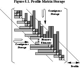
At about the same time, R. C. Young, a mechanical engineer at General Atomic, saw the AP-120B architecture as potentially useful for the three-dimensional structural analysis problems that were out of the range of conventional machines. But the precision needed to be a bit higher, and some way had to be found to achieve the effect of a large virtual address space so that the many megawords representing the stiffness matrix could be handled without slowing computation. The latter problem he solved by using a block factorization technique that overlapped disk fetches with submatrix multiplications. As discussed in Section 5.5.4 below, M by M matrix multiplies can perform M multiply-adds for every input data value, so a disk 50 times slower than the arithmetic unit (0.2 to 0.3 MWords/second versus 12 Mflops) can still keep pace once the stiffness matrix, stored with profile sparsity, has an average profile on the order of 50 elements (See Figure 5.1).
Both Kenneth Wilson’s and R. C. Young’s efforts influenced the next generation of array processors, typified by the FPS-164. The FPS-164 had full 64-bit precision words, more registers, a somewhat more complete crossbar between functional units to assist Fortran compilation, and greatly expanded memories throughout the system. Since it ran entire Fortran programs instead of subroutines, its environment resembled that of the CRAY-1 more than that of the AP-120B, and the term “attached processor” was used to denote this distinction from “array processors.” The applications that follow are appropriate for attached 64-bit processors.
5.3.1 Structural Analysis
Structural analysis is used to predict the behavior of objects ranging from tiny machine parts to bridges and large buildings. Its numerical methods are mature, and are not confined to stress analysis but can also calculate heat flow or electromagnetic fields to very high accuracy. It relies on the “Finite Element Method,” whereby the structure is broken into geometrically simple domains called “elements” for which an exact analytical solution exists. The global solution is found by mating element boundaries together in a consistent way, which amounts to the construction and solution of a large system of equations called the “global stiffness matrix.” For sufficiently large models, factoring the global stiffness matrix dominates run time.
With the exception of the matrix setup and factoring, structural analysis is very much a problem for general-purpose computers. A structural analysis program like MacNeal-Schwendler’s MSC/NASTRAN involves hundreds of thousands of lines of source code, and spends much of its time moving data from disk to memory and back with very little arithmetic. Structural analysis environments must support interactive graphics terminals, data formatting, low-precision integer operations, archiving to disk and tape, and other functions for which very few compute-intensive processors are economical. The solution, then, is to combine a general-purpose computer with some sort of arithmetic enhancement to try to make the matrix solution time commensurate with the time spent on the rest of the task. IBM introduced its vector facility for the 3090 mainframe with this situation in mind, and attached processors such as the FPS-164 and FPS-264 can economically handle all but the preprocessing and postprocessing parts of the run, leaving those to an IBM or VAX host.
To illustrate the magnitude of the matrix solution step, suppose one wishes to model a cubical elastic body divided into cubical elements, 100 on a side. Each cube corner has three translational and three rotational degrees of freedom, so there are roughly 6 x 10⁶ unknown quantities to be solved for. If the elements are numbered lexicographically, the matrix describing the system has a bandwidth on the order of 104, and the solution of the matrix for a single set of input forces takes about 1013 floating point operations. A machine with an effective speed of 10 GFLOPS would therefore take fifteen minutes to compute a single static response, and T times that if T timesteps are desired for a dynamic analysis. So structural analysis is appropriate for compute-intensive processors, especially for the larger problems; the percentage of the total work spent in the matrix solution phase approaches 100% as problems grow large in the number of elements.
5.3.2 Analog Circuit Simulation
The SPICE circuit simulation emerged as a public-domain program from Berkeley around 1972, and has since undergone much modification and commercialization. Early users of SPICE soon discovered that it was not the least bit difficult to find relatively simple circuits for which SPICE runs appeared interminable on general-purpose machines.
SPICE does its own memory management from within Fortran, dimensioning all of available memory as a single array, and using integers as pointers to allocate and de-allocate regions of memory at run time. The dynamic sizing of arrays that this permits is essential for circuit simulation, since it is difficult to estimate memory requirements before the run begins. This memory management from Fortran severely burdens the memory bus of a computer, and speed at SPICE is all too frequently a function of the MBytes/second rating of the memory and the latency of the memory. Latency is critical because the memory management adds a level of indirection to the memory references. Pipelined memory is of little help for conventional SPICE, which was written well before the advent of compute-intensive processors.
The elements of the circuit have current-voltage properties that require substantial calculation; a transistor element evaluation might involve several pages of source code containing exponentials, tests, branches, polynomial evaluations, and square roots. Machines with data caches such as the VAX perform relatively well on SPICE, since modeling each element means bringing in a small amount of memory and using just that memory intensively. The original version of SPICE makes no attempt to group devices by type so as to permit vectorized evaluation; vectorized versions for compute-intensive processors such as CRAY and the FPS-264 group the devices, use conditional merges to replace branching, and work very well on large-scale circuits where there is a great deal of repetition of device type.
Analog circuit simulation spends most of its time alternating between the setup of a large, very sparse asymmetrical matrix, and solving that matrix. An element of the matrix Aij is nonzero if circuit element i is connected to circuit element j. Circuit elements such as diodes create asymmetries in the matrix, so the economies of symmetric matrix factoring are not available to most circuit models. Before factoring, there might be only five or six nonzeros per row of the matrix, in a matrix several hundred elements on a side. A symbolic factoring determines where nonzeros will arise in solving, and that symbolic factoring needs updating infrequently relative to the number of times the matrix is actually solved; the cost of accounting for the sparsity is amply repaid after a few iterations. This is a very different approach to matrix solving from the dense or banded systems discussed above; a profile-type approach, even on specialized hardware (see Section 5.6.2) does not seem to overcome the advantages of exploiting sparsity.
On a general-purpose processor, the division of time between matrix factoring and matrix setup (device property evaluation) is roughly half and half. On a compute-intensive processor, the division is more like 20% for the factoring and 80% for the setup! It is worth noting that a vectorized version of SPICE for the CRAY-1 only achieves about 100 times the speed of the VAX-11/780, despite the much higher ratio (about 1000:1) in peak 64-bit arithmetic speed. Analog circuit simulation, even when substantially reorganized from the Berkeley version, is memory-intensive and best handled by compute-intensive processors that have a very short path to main memory.
5.3.3 Computational Chemistry
There are many ways that computers can be used to simulation the behavior of chemical entities, ranging in complexity from a simple hydrogen-hydrogen bond to the dynamic behavior of a strand of DNA with dozens of component atoms. In general, the simpler problems are studied with ab initio methods based on the laws of quantum mechanics, whereas more complicated molecules must make use of approximations in order to render the problems computationally tractable. The electrons in a molecule have several energy states that can be approximated as a combination of “basis functions.” The basis functions are analogous to the polynomial terms in a Taylor series expansion, and when chosen appropriately form a complete set for describing the molecular bonds.
Ab initio methods compute the interaction of electron states, ignoring those below a certain energy threshold. With N basis functions, the number of interactions is O(N4). The interactions, or “Gaussian integrals,” typically number in the billions and must be stored on disk rather than in main memory. An O(N5) or O(N6) process, involving eigenvalue extraction, then produces the configuration of basis functions that best describes the molecule.
The process is well-suited to compute-intensive processors, with one exception to the paradigm; the primary feature required other than 64-bit floating point operations is the ability to move data quickly to and from secondary storage, with large secondary storage. Some compute-intensive processors can recompute the Gaussian integrals faster than they can be retrieved from disk, thereby eliminating the need for a large and fast secondary storage. There is also need for logic and bit-packing operations, since the indices of an integral are usually packed into a word to save storage.
The processing of the integrals usually involves repeated matrix multiplications, the canonical operation of compute-intensive processors. If the architecture can efficiently exploit sparsity, then there are great performance benefits, because a typical matrix in computational chemistry only has 10% nonzero elements. A 10% sparse-10% sparse matrix multiply requires, on the average, only 1% of the multiply-adds of a dense-dense matrix multiply, so the potential speedup is on the order of a hundredfold. One approach, known as “Direct Configuration Interaction” (CI), consists almost entirely of matrix multiplication, which was a motivation for the FPS-164/MAX special-purpose architecture (see Section 5.6.2).
5.3.4 Electromagnetic Modeling
For pure number-crunching, few applications can compare with that of assessing the radar reflection of a metal object such as an aircraft. Because every point on the metal object acts both as a receiving antenna and a re-radiating antenna, every point affects every other point, so the equations describing the problem are dense. It is not unusual to have to factor and solve a dense, complex-valued set of 20000 equations in 20000 unknowns, requiring over 20 trillion floating point operations and over 6 billion bytes of (secondary) storage! The result of the computation is the “cross-section” seen by a detector from various viewing angles.
Even the most highly-specialized compute-intensive processor can be used efficiently on the radar cross-section application. The vectors are long, hundreds of operations are performed for every communication of data to or from disk, and the inner loop of the factoring is pure multiply-add arithmetic: a complex dot product. Setting up the matrix is a more scalar-intensive operation, but is usually less than 1% of the total work. The problem must be done with 64-bit precision; the problem can be formulated as an ill-conditioned matrix of modest size or a numerically better-behaved matrix of the size mentioned above. In either case, less than 64-bit precision does not seem to lead to useful answers.
5.3.5 Seismic Simulation
The oil exploration industry uses 32-bit processors to analyze seismic measurements and form hypotheses about what is underground. Because the problem is severely underdetermined, choosing from among many possible underground formations remains an art as much as a science. A natural method for checking the hypotheses is to ask a computer the following question: If this particular structure describes what is underground, what would have been detected by the seismic sensors? Answering this question requires a 64-bit simulation, the opposite the data acquisition problem. It is conceptually simple. One describes the rock layers in the computer memory by position and refractive index, produces a point disturbance at the memory location representing the “shot point,” and then uses a difference equation to simulate the wave that propagates through the earth. The values in storage locations representing the surface of the earth simulate the displacements that would be recorded by seismic detectors.
In the “acoustic model,” there is only one degree of freedom at each discrete space point, representing pressure. A far more accurate method recognizes the earth as an elastic medium, with independent stresses and torques in every dimension. The elastic model uses principles from Finite Element Methods, but avoids factoring a global stiffness matrix at every timestep; each degree of freedom can be computed explicitly from the nearby data of the previous timestep, since stresses cannot propagate faster than the speed of sound in the medium. Problem size is usually limited by main memory size, since a full elastic three-dimensional model N by N by N model requires two timesteps in memory, each with 6N3 64-bit words of main memory. Current supercomputers are inadequate for models with completely satisfactory fidelity. In general, the problem is ideally suited to the compute-intensive paradigm.
5.3.6 AI Applications
The main AI applications for compute-intensive processors is in recognition of sounds and images. Understanding the sound or image is a very different problem, requiring more of a Lisp-type environment that is not at all dependent on arithmetic.
As an example, speech recognition involves both identification of phonetic sounds (independent of speaker) and mapping those sounds to the most probable word in the language. Assessing the meaning of the speech is a separate phase, although feedback from that understanding can assist future recognition by adjusting probabilities and weighting factors assigned to raw input data.
Another example is satellite image processing. A large amount of arithmetic computation goes into refining data from satellites prior to being able to use AI methods to distinguish structures (e.g., airbases from highways, tanks from trucks). An array processor might well be coupled to a Lisp-specific computer to handle both parts of the task with specialized hardware.
Finally, an example of a compute-intensive AI application is that of the “Neocognitron” neural network model for visual pattern recognition developed by Nippon Telephone and Telegraph researchers. It refines handwritten Arabic numerals described on a 19 by 19 array of pixels through twelve stages to a final 1 by 10 array representing digits 0 to 9. By “teaching” the network using a small number of distorted examples, the Neocognitron can accurately recognized a wide range of written numerals. Each “neuron” performs essentially a floating point inner product followed by a binary decision, with a very high ratio of computation to communication. Since neurons are known to integrate information that is digital in amplitude but analog (best represented by floating point numbers) in time, it seems likely that compute-intensive processors will play a role in AI applications based on neural networks.
5.4 Design Philosophy
General-purpose computers do surprisingly little arithmetic. The majority of instruction cycles in the world are spent moving data from one place to another without performing operations on them. A typical example is word processing. String comparison and computing the best location of text on a page are virtually the only arithmetic tasks involved; the rest of the work consists of moving information between keyboard, memory, display, printout, and mass storage. Most of the capital investment today in computers is in mainframes oriented toward business applications. These are used for searching through disks and tapes for information, sorting, and tracking events (such as banking transactions or airline reservations), all of which involve an occasional byte-level comparison or fixed point (integer) calculation. But in fact arithmetic is relatively rare, and high-precision floating-point arithmetic is practically unused on such machines except in figuring compound interest! For good reasons, then, conventional computers are designed with communication and storage of data foremost in mind.
Table 5.1 illustrates this fact using a list of the most-used instructions on the venerable IBM/370 family [IBM 86]:
Table 5.1 IBM/370 Instruction Frequencies
% of Total
Instruction Instructions
Branch on Condition 20.2
Load from Memory 15.5
Test under Mask 6.1
Store to Memory 5.9
Load Register 4.7
Load Address 4.0
Test Register 3.8
Branch on Register 2.9
Move Characters 2.1
Load Halfword 1.8
This “top ten” list accounts for 66% of the instruction usage on the IBM/370, but contains not a single mathematical operator. A similar study has been done for Digital Equipment’s VAX-11/780:
Table 5.2 VAX-11/780 Instruction Frequencies
% of Total
Instruction Type Instructions
Simple (Moves, etc.) 83.6
Bit Manipulation 6.92
Floating Point Math 3.62
Call/Return 3.22
System Management 2.11
Character Manipulation 0.43
Decimal Instructions 0.03
Scientific and engineering applications are such a sharp contrast to this distribution of instruction usage that they demand an entirely different approach. These applications are typically heavily laden with arithmetic operations. When run on a general-purpose machine without floating-point hardware, most of the time will be spent in the software or firmware routines that combine basic integer operations to accomplish a floating point operation. Time spent fetching data becomes negligible by comparison, leading to algorithms that minimize total work simply by minimizing the number of floating point operations.
Extensive hardware is necessary to reduce floating point calculation time to a few processor clock cycles. Such hardware can roughly double the number of gates in a processor! Since doubling gate count might nearly double hardware cost, manufacturers of general-purpose computers prefer to leave out such hardware since most of the their customers would never use it, and would find such machines less cost-efficient for business tasks.
This dilemma has brought about the separation of computers into two classes: those optimized for business processing, typified by the mainframes built by International Business Machines, Unisys, and Digital Equipment, and those optimized for scientific processing, typified by mainframes built by Control Data and Cray Research. An alternative approach is a compute- intensive processor that attaches to a general-purpose mainframe to provide floating point speed via an optional peripheral device. These attached processors, typified by those made by Floating Point Systems and Star Technologies, are able to leave out many hardware functions that are taken care of by the host processor, recovering cost-efficiency that would otherwise be slightly worse than a solution based on a single scientific processor. Figure 5.2 illustrates the tradeoff between generality and compute-intensive efficiency:
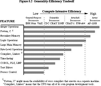
The CRAY-1 is very nearly in the attached processor class, requiring a host processor to manage it but differing from attached processors in that it runs its own compiler and linker. At installations where CRAY usage is heavily subsidized, complete time-sharing and even text editing are done directly on the compute-intensive processor despite the very poor cost-efficiency of that approach.
A glance at the instruction set for a general-purpose computer reveals operations for converting binary number representations to character representations, rotating and shifting the bits of words, and prioritized interrupt handling to assist in sharing machine resources among multiple users. Compute-intensive processors can have greatly simplified designs through the elimination of such instructions. Where necessary, those functions can be built somewhat inelegantly from other operations, just as some general-purpose processors build floating-point operations. A compute-intensive processor will typically have instructions such as floating-point multiply, add, subtract, reciprocal (not necessarily a divide!), square root, and conversions between floating-point and integer representations.
Besides the presence or absence of instructions, compute-intensive processors have very unusual ratios of communication speed to computation speed. On general-purpose machines, it typically takes one or two orders of magnitude longer to perform a floating-point operation than to fetch or store the operands/result; on compute-intensive processors, the ratio is closer to unity. We will later discuss an example in which 248 floating-point operations occur (usefully) in the time required for a single memory reference! In the case of a polynomial evaluation, computing the norm of a vector, or multiplying a matrix times a vector, the ratio of speed for
Memory Reference : Floating Point Add : Floating Point Multiply
can in fact be 1:1:1. Most compute-intensive processors approximate this ratio. Examples include the FPS-264, the CRAY-1 (but not the CRAY X-MP), the Convex C-1, and the Alliant FX series. The CRAY X-MP actually has multiple ports to main memory, making its ratio 3:1:1 and tending toward more general-purpose computing.
5.5 Architectural Techniques
Although the last 50 years of computer technology show steady and dramatic improvements in cost, size, speed, and packaging, history repeats itself with respect to computer architecture. The board-level processors of the 1970’s rediscovered techniques of the mainframes of the 1960’s, and in the 1980’s those techniques have been discovered yet again in single-chip processors. For example, the concept of multiple pipelined functional units appears in the CDC 6600 mainframe, then the AP-120B array processor, and today in chip sets such ase the 2264/2265 from Weitek. Several vendors are currently working on consolidating a multiple-pipeline compute-intensive processor onto a single VLSI chip. The designers of compute-intensive processors, whatever the technology or scale, have repeatedly faced the same issues:
• How many different functional units should there be?
• How can they be controlled by an instruction stream?
• How much parallelism can be used by Fortran-type environments?
• How much main memory is needed to keep the processor busy?
• Can registers or cache successfully substitute for main memory?
• What is the optimal ratio of vector speed to scalar speed (pipeline length)?
• What is the ideal precision (32-bit, 64-bit, etc.)?
The following sections offer some arguments that have been used in successful designs, illustrating tradeoffs that must be made.
5.5.1 Functional Units
The idea of multiple functional units dates back at least to the ATLAS computer of the early 1960’s. Separate functional units for memory addressing and register-to-register operations are nearly universal. On a compute-intensive processor, one might envision so many different functional units that a Fortran expression such as
A(I,J) = 0.5*(SQRT(FLOAT(I/2)))*B(J)+3.0/C(I,J)
could be evaluated efficiently by having a processor that contains a machine for the integer divide , a machine for the FLOAT, a machine for the SQRT, two floating-point multipliers, a floating-point divider, a floating-point adder, and address calculation units for the (I,J) indexing, all capable of cooperating on this task! Hardware cost grows with the number of functional units, faster than linearly because of the need to heavily interconnect the functional units (the classic crossbar switch problem). Studies of compute-intensive kernels [Charlesworth 81] reveal that a typical mix of operation is weighted as
Operation Relative Weight
Operand Reference 7
Integer Add/Subtract 1 to 2
Integer Multiply < 0.1
Floating Point Add/Subtract 1
Floating Point Multiply 1
Divides < 0.1
Square Roots < 0.1
It is an engineering heuristic that a processor is most cost-efficient when no single part is a conspicuous bottleneck. Therefore, the preceding list implies that a well-balanced compute- intensive processor should have an integer adder, a floating point adder/subtracter, a floating point multiplier, and should handle the other operations less directly. For example, divides can be accomplished (with a slight increasing in rounding error) by fetching a reciprocal approximation of the denominator from a table in Read-Only Memory, refining the precision with Newton-Raphson iterations (using the floating point Adder and Multiplier), and finally multiplying by the numerator. This is perhaps an order of magnitude slower than an add or multiply, but is acceptable for the typical mix of operations shown above.
The list also indicates that there should be the ability to fetch or store about seven operands for every time the floating point multiplier and adder units complete an operation. But doing this from main memory is exactly the communication cost that compute-intensive processors seek to avoid! Since the adder and multiplier each take two inputs and produce one output, it is evident that at least six operand references are necessary to sustain anything close to the peak speed of the arithmetic. The solution usually makes use of registers and the interconnect between functional units rather than memory bandwidth, the most limited resource in a von Neumann design. For example, a processor could provide two register reads, two register writes, a main memory reference, a local “table memory” reference, and connect the output of one floating-point functional unit to the input of another, providing a total of seven operand references, of which only one actually burdens the main memory bus.
5.5.2 Processor Control
When is such a processor supposed to obtain instructions, with memory tied up moving data? A separate program store is called for, either as a cache or a memory explicitly loaded by the user. Program caches can be much simpler than data caches, since there is usually no requirement to write to a program cache during a run, which eliminates the need for the cache to ever write anything back to main memory. They also can be fairly small, since compute-intensive applications usually involve small loops occupying less than 1K of program store. Opportunities to fill the cache from main memory arise whenever serial data dependencies allow the data reference unit to go idle. Alternatively, one can simply have a separate memory for program storage that must be loaded explicitly. Caches are characteristic of attached scientific computers that must run entire Fortran programs, whereas separate program stores are characteristic of array processors that concentrate on simple subroutines.
There is a price to pay for the multiple instruction units in the instruction word. The choice is to either “hard-wire” a set of basic operations such as dot product, vector add, etc., and use the instruction to select one of those basic operations, or else provide a wide instruction word that explicitly controls all of the functional units with parcels of bits within the instruction. Programming the latter has an analogy with the task of writing multipart musical harmony. The rules of Western music place certain context-dependent restrictions on what notes can occur simultaneously, and voices enter the harmony depending on what has come before, just as incomplete crossbars limit what operations can be performed simultaneously, and just as loop iterations imply an order in which functional units can be invoked. Constructing a software pipeline for a simple vector operation can be every bit as difficult as writing a canon or round. Consider a loop for computing an inner product
DO 10 I=1,N
10 SUM = SUM + A(I) * B(I)
and the round, “Row, Row, Row Your Boat”:
Fetch A(I) Row,
Fetch B(I) Row,
(Memory pipeline wait) Row, Your Boat,
(Memory pipeline wait) Gently
Multiply A(I) and B(I) Down the
(Multiplier pipeline wait) Stream…
(Multiplier pipeline wait) Merrily,
Add product to SUM Merrily,
(Adder pipeline wait) Merrily, Merrily,
Test I=loop end? Life is
(Comparison wait) but a
Jump to beginning Dream. (Repeat)
Both the program and the music have been arranged in such a fashion that a conflict-free pipeline can be established, as shown in Figure 5.3:
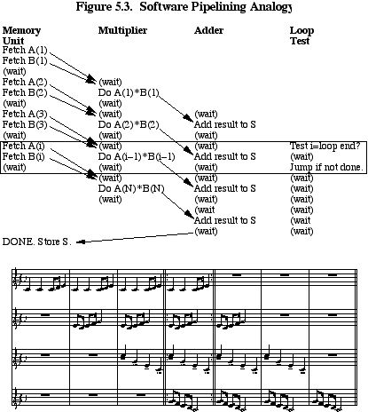
Note that the role of the singers in the music above is not the usual one where each singer repeats the entire melody; the notes that occur are identical if each singer behaves as a “functional unit” for a single phrase. Whereas many people can write a melody, very few can write multiple melodies that interlock properly as a fugue, and still fewer can create a melody the interlocks properly when overlapped with itself! For this reason, compute-intensive processors with simultaneous control of many functional units have a reputation of being much more difficult to program efficiently than conventional machines. Surprisingly, a Fortran compiler can generate conflict-free schemes such as that shown above. A pipelining compiler was first introduced in 1983 by Floating Point Systems [Touzeau 84]. The problem of scheduling the units for optimal efficiency is known to be NP-complete, so the current version of the compiler only performs a shallow search of the tree of possibilities. Empirically, this turns out to produce efficiency comparable to that of hand-tuned assembly code. This type of compiler is markedly different from “vectorizing compilers” targeted at vector processors.
On a “vector processor,” the type of loop shown above would be in microcode that the user can invoke but never alter. This greatly reduces the burden on the instruction bandwidth, but restricts the set of operations. For example, to perform a sparse dot product of the form
DO 10 I=1,N
10 SUM = SUM + A(J(I)) * B(I)
is only slightly more work for a software-pipelined machine, but at least twice as hard for a vector machine that must construct the operation from a Vector Gather followed by a Vector Multiply Reduction Add. The compiler burden shifts to one of recognizing vector forms expressed as DO loops by template matching; the compiler must then attempt an efficient construct from the basic forms available on the machine. The hardware to manage vector forms is expensive, but so is programming assembly language on a software-pipelined machine. The argument has yet to be firmly settled in the community of computer users.
5.5.3 Parallelism and Fortran
Fortran, despite its historical development as a language for serial architectures, shows a fair amount of functional parallelism close to the surface. If a Fortran text is divided into “basic blocks,” that is, code segments bounded by subroutine calls or branches, then the program text implies a data dependency graph that can be extracted by an optimizing compiler. In the case of DO loops where iteration n+1 is independent of iterations 1 to n, there might well be as many concurrent operations in the data dependency graph as there are iterations of the loop. For example, the vector add
DO 10 I=1,N
10 R(I) = A(I) + B(I)
involves N completely independent additions. Optimization for this goes hand-in-hand with the multiple functional unit idea, since the units can be scheduled at compile time. Many general-purpose computers use concurrency only at run time, where the processor looks ahead in the instruction stream and tries, for example, to pre-fetch operands that will soon be needed while some other operation is completing.
The philosophy in compute-intensive processors has traditionally been to put the burden on the compiler or other software tools such as libraries of vector operations, thereby lessening the amount of hardware needed to detect and make use of concurrency at run time. This affects the Edit-Compile-Link-Run-Debug cycle in which the user sits, because on small problems the time saved in the Run will be consumed by the additional time during the Compile. For this reason, attached processors and array processors are inherently less interactive than general-purpose computers when traditional programming languages are used.
5.5.4 Main Memory
Asked why his computers do not have virtual memory, Seymour Cray reputedly once said, “In machines this fast, there’s no use pretending you got something you ain’t.” Compute-intensive processors do not spend a great deal of time operating on any one page of memory, nor do they go for long periods without a memory reference during which a data cache can be moved to or from disk storage. Thus, the strategy is usually to have a large physical memory, making the best use of address bits by addressing words, even 64-bit words, rather than bytes.
How big should the main memory be? This is highly application-dependent, but the answer stems from the need to amortize the time to load and unload the data for a particular problem. If it takes five seconds to load a program and its data set, then the computation should take at least as long. Although initialization grows linearly with the amount of memory to move, the amount of computation usually grows superlinearly. For example, an N by N matrix multiplication requires 2N2 input values but 2N3 operations, so for some sufficiently large N, the system will spend most of the time computing rather than communicating data. As a specific example, suppose that the loading proceeds at 0.1 MWord/second, and the compute-intensive processor can perform 10 million floating point operations per second. If we require communication time to be roughly 1% of the total, then
Load Time = Compute Time / 100
which implies that
(2N2 words)/(0.1 MWords/second) = (2N3 operations)/(10M operations/second) x 1%
This is satisfied when N is 10000 words. This is quite a bit smaller than the typical memories of general-purpose processors, suggesting that for some applications, simple array processors can improve cost efficiency by reducing main memory size. Attached scientific computers must have larger memories since they contain the entire application program (or large overlays of it), not just compute-intensive kernels, and must use physical memory rather than virtual memory for both program and data.
General-purpose computing is characterized by problems for which the number of computations grows proportionately to the amount of data If desired run time is on the order of seconds, then a general-purpose processor capable of X operations per second should have about X words of memory. The above argument, however, shows that compute-intensive processors can often succeed with less than this. The CRAY-1, for example, is capable of over 150 million floating-point operations per second, yet has only 1 million words of memory. The reason behind this is that scientific computing is characterized by problems (such as matrix multiplication) for which the number of computations per data point grows much faster than the number of data points.
5.5.5 Registers
Since data caches appear difficult to make efficient for the whole spectrum of memory reference patterns used for compute-intensive processing, one must have a large set of registers close to the functional units. For example, the FPS-164 has 64 integer registers and 64 floating point registers, with the capacity for several simultaneous reads and writes per clock cycle. The CRAY-1 uses multiple vector registers, where each vector contains 64 floating point elements, to keep operands within a few nanoseconds of the functional units. Besides the obvious design difficulties and parts cost of having a large number of fast registers, state-save becomes much slower, making context-switching a clumsy operation. Compute-intensive processors are thus not intended for time-slicing between multiple users, at least not with time slices measured in milliseconds! (Hardware to partition registers as well as memory among multiple users is generally counter to compute-intensive design). They also have trouble with languages such as Ada and Pascal, for which subroutine calls require an extensive state-save.
5.5.6 Vector-Scalar Balance
A “vector operation” is an operation that is repeated on a list of numbers; a “scalar operation” is an operation on a single number (one-argument functions) or pair of numbers (two-argument functions). (Unfortunately, the terms “parallel operation” and “serial operation” are often mistakenly used as synonyms for “vector operation” and “scalar operation”.) Vector arithmetic is efficient because it allows the re-use of an instruction and because it permits a hardware pipeline to process the vector in a manner analogous to an assembly line. An excellent survey of pipelining techniques and history can be found in [Kogge 81].
If a pipelined functional unit has N stages, then a scalar operation on that unit will take N clock cycles to complete and be N times slower than the speed for long vectors where a result is completed every cycle. There will also be N–1 latches between stages, and hence pipelined units are slower at scalar operations than simple scalar units. The tradeoff for the computer designer is to strike a balance that prevents either scalar-type or vector-type operations from showing up as a performance bottleneck.
Suppose, statistically, that 75% of an application is vector-oriented and the rest is scalar, as timed on a completely scalar processor. Then a machine that is three times faster at vector processing than scalar processing will spend equal time in both types of code, and neither will appear as a bottleneck. If the same functional unit performs both scalar and vector operations, then the use of 3-stage pipelines is suggested. If 90% of the application is vector-oriented, one would wish for 9-stage pipelines, although there is a limit as to how finely one can pipeline tasks like multiplication and addition! One manufacturer of array processors, CSP Inc., discarded the idea of pipelining entirely, with the argument that scalar units are easier to compile to. FPS opted for pipeline lengths of 2 or 3 stages in the functional units of the AP-120B and FPS-164 processors, and the pipelines in the CRAY-1 are up to 14 stages long. The memory pipeline on the original CRAY-2 is roughly 60 stages long, which is perhaps a record. Applications are generally scalar-bound on such machines. The CRAY machines generally fit the definition of a compute-intensive processor, since a scalar floating-point operation is faster than a memory reference, and vector memory bandwidth (full pipelines) is just fast enough to keep up with the peak speed of the vector floating-point functional units.
The current generation of VLSI floating-point parts uses mostly four-stage pipelines for the multiplier and adder. Note that it is convenient to have the number of stages be a power of two, since if there are 2n stages then binary collapses can be efficiently done in n passes for reduction operations such as sums and inner products.
The term “array processor” stems from the fact that these small, simple compute-intensive processors are frequently used to perform highly repetitive operations on arrays of numbers, but in fact the term is misleading. Pipelines in array processors are shorter than in supercomputers, making them actually better adapted to scalars and short vectors, and to programs with recursion and branching. Perhaps “subroutine processor” would be a more accurate term, since the main distinction between array processors and supercomputers is the generality of their capabilities (as shown in Figure 5.2.)
5.5.7 Precision
When floating point operations are constructed in software from integer shifting and summing operations, 64-bit operations take almost twice as long as 32-bit operations. In hardware, 64-bit operations can be brought down to approximately the same length critical path by adding extra gates and increasing the width of data paths. But a machine with 64-bit words and only full-word addressing must have double the storage cost for a 32-bit application.
Attached processors have the additional problem that users are generally unwilling to tolerate either loss of precision or loss of dynamic range in passing data from the host to the attached processor. Therefore, an attached processor should have at least as many mantissa bits and at least as many exponent bits as every host to which it will be attached! In the AP-120B, this led to the choice of a 38-bit data word since there were so many floating point formats in use by various vendors for “single-precision” (usually 32-bit or 36-bit) data. As more 32-bit machines standardize on the IEEE floating point standard and 36-bit computers become less common, more attached processors are able to use VLSI parts based on the 32-bit IEEE format without encurring loss of precision or range through data transfer.
Required precision is a function of application. Some generalizations are listed below:
32-bit precision: 64-bit precision:
Most signal processing Structural analysis (Finite Element Methods)
Most image processing Circuit simulation (stiff ODE’s)
Lattice-gauge calculations Ab initio computational chemistry
Missile simulation (simple ODE’s) Electromagnetic wave modeling (inverse problems)
Most graphics (rendering) Seismic simulation (forward modeling)
Seismic migration High-order or hyperbolic finite difference schemes
Coarse-grid, elliptic Computational fluid dynamics
finite difference schemes Oil reservoir simulation
Data acquired from physical phenomena (seismic data reduction, satellite image processing) rarely have more than four decimals of precision or four orders of magnitude dynamic range, and hence signal and image processing usually need no more than 32-bit precision
Lattice-gauge simulations are unusual among compute-intensive simulations in that errors accumulated using 32-bit arithmetic on small unitary matrices can be periodically removed by renormalizing to keep determinants close to unity.
Missile simulation and other models involving Ordinary Differential Equations (ODE’s) with few degrees of freedom frequently have very stable numerical methods, and errors caused by use of single precision damp out over repeated timesteps.
Rendering methods for generating photographic-quality simulated images (such as ray-tracing) need only compute with the precision that will be relevant to a raster-scan display (about one part in 1000). An exception occurs when one must compute the intersection of nearly parallel plane sections, which is an ill-posed problem mitigated by judicious use of 64-bit precision.
Finite difference schemes for solving Partial Differential Equations (PDE’s) often have inherent numerical error proportional to some low power of the grid spacing. For instance, the usual five-point operator applied to an n by n grid only has accuracy proportional to 1/n2, so one usually runs out of memory and patience when n is increased before one runs out of precision! This applies to static problems such as elliptic PDE’s where errors do not propagate with time.
Structural analysis methods use finite element methods, which are in principle far more accurate than typical finite difference methods. A large problem might lose seven or eight digits in the process of solving the global stiffness equations, however, so 64-bit precision or better is essential. The need for high precision is easily seen by considering the bending of a beam: although the overall bending might be quite significant, the strain on an element in the beam is perhaps one part in a million. Since the overall bending is computed by accumulating element strains, small errors caused by precision translate into major macroscopic errors.
Analog circuit simulation can easily run into ill-posed sets of nonlinear ODE’s for which high precision helps convergence. Iterations can get “stuck” on the jagged steps of 32-bit precision, even though far from the best solution of the nonlinear system.
Computational chemistry involves the computation of eigenvalues (which represent energy levels of molecular orbitals) where the eigenvalues span many orders of magnitude, and operations on matrices where the sum of many small quantities is significant relative to a few large quantities; some computational chemists are even forced to use 128-bit precision, for which hardware support is rare.
Electromagnetic wave modeling, used to simulate radar reflections from metal objects, is currently done using boundary integral techniques that give rise to very large (10000 by 10000) dense systems of linear equations; since the bound on roundoff error is proportional to the number of equations times the relative error of the floating point representation, 64-bit precision is preferred.
Seismic simulation is a large hyperbolic PDE model, not to be confused with seismic migration. One is the inverse of the other. Fine-grid finite difference schemes involving multipoint operators can be accurate enough that single-precision floating point error exceeds the error of the numerical method; hence double precision is needed.
Oil reservoir simulation at first glance appears feasible using 32-bit precision, since coarse grids are used; however, the methods repeatedly calculate pressure differences at adjacent grid points, where subtraction of large similar uncertain numbers removes many significant figures.
In summary, there are a variety of reasons why high-precision arithmetic might be needed by an application. As models become larger or more detailed, some low-precision applications are moving into the high-precision camp.
5.5.8 Architecture Summary
Table 5.3 summarizes tradeoffs for various compute-intensive architectural techniques:
Table 5.3 Architectural Tradeoffs
METHOD ADVANTAGES DISADVANTAGES
Multiple Higher peak speed; Extra hardware cost;
functional better cost/performance; complicated control needed;
units widely applicable hard to program efficiently
Wide Customizable to application; Must decode at run time;
instruction efficient compilation possible; high program bandwidth needed;
word allows fine-grain concurrency optimal scheduling difficult
Virtual Applications run regardless Typically high cache miss rate
memory of actual memory configuration greatly degrades performance
Large Less memory speed burden; Expensive state-save;
register allows “scratchpad”-type expensive hardware;
set programming at high speed slow context switching
Vector Much higher peak performance; Complicated to build;
arithmetic somewhat higher typical pressures users to alter programs;
performance reduced scalar speed
Many opera- Very high peak Mflops; Very application-specific;
tions per less memory speed burden; pressures users to alter programs;
instruction rewards organized programs poor at branching, calls
High- Wider range of applications Increased memory size needed;
precision run satisfactorily; greatly increased hardware;
word size less roundoff expertise needed waste on low-precision
operations
5.6 Appropriate Algorithms
The body of knowledge about numerical algorithms that has formed over the last forty years has largely been based on the assumption that calculation is expensive and memory references instantaneous and free. On general-purpose computers, this is still sometimes a good approximation to the truth; for example, personal computers (without coprocessors) typically take 100 to 1000 times as long to do a 64-bit floating point multiplication as to simply fetch a 64-bit word from memory. Unfortunately, compute-intensive processors bring the ratio close to unity, so traditional analysis of computational complexity is frequently inadequate when attempting to select an appropriate algorithm for attached processors or array processors.
5.6.1 Dense Linear Equations
Consider the classic problem of solving a system of equations represented by Ax = b, where A is a dense, real, n by n matrix, x is the unknown n-long real vector, and b is a given n-long real vector. A typical implementation of Gaussian elimination might resemble Algorithm A:
A1. For column k = 1 to n–1:
A2. Find the element Aij in the column with the largest magnitude (pivot).
A3. Exchange the row Ai* with row Ak* so the pivot is on the diagonal.
A4. For row i = k+1 to n:
A5. Compute R = Aik / Akk .
A6. For row element j = i to n:
A7. Compute Aij – R .Akj and store in the Aij location.
A8. Next j.
A9. Next i.
A10. Next k.
The usual work estimate for this algorithm is 2/3n3 + 2 n2 + O(n) floating point operations. Line A7 is executed 1/3n3 times and constitutes the kernel of the algorithm. Now consider the memory burden imposed by that kernel. The computer must reference Aij , Akj , and then Aij again for each multiply-add; R is easily held in a register. If a compute-intensive processor can only make one main memory reference per multiply-add, it will be limited to only 1/3 of peak speed in this algorithm. Furthermore, the references in the kernel use pointers to the two sets of locations Aij … Ain and Akj … Akn, which for column storage means incrementing pointers by a constant stride of n. This requires an integer addition, which is usually more expensive than increments by unity. In addition to the two constant strides, an integer add is needed to test the loop for completion, also limiting the kernel to 1/3 of peak.
The simple act of reordering the operations by changing loop nesting in the preceding algorithm can remove this problem. By arranging the loop over k to be the innermost loop, the kernel can be changed to an inner product, as shown below for the inner two loops:
B1. Save Aij in a table memory, yi (contiguous).
B2. For j = i to n:
B3. Set S = 0.
B4. For k = i to n:
B5. Set S = S + yk .Akj
B6. Next k.
B7. Scale by diagonal pivots.
B8. Next j
The kernel, line B5, can keep S in a register and yk in a vector register or table memory. The yk quantities are used O(n) times, effectively spreading the cost of the main memory reference to load them into the vector register. There is only one memory reference in the kernel, that of Akj, that uses a contiguous stride through a column of matrix storage. Hence the kernel involves a register add, a floating point multiply, and an integer comparison for the end-of-loop test. This can execute at near-full speed on most compute-intensive processors; hence, there is at least one useful application that allows this type of computer to approach its claimed performance for periods of at least several seconds rather than just a burst of a few microseconds. A more detailed discussion of this problem can be found in [Dongarra 84].
If the floating point adder is pipelined with p pipeline stages, the S accumulation will actually be done as p subtotals moving through the pipeline. The inner product y* .A*j actually becomes a matrix-matrix multiply where y is a matrix with p rows, yielding p subtotals that are collapsed later. Note that this affects the floating point roundoff error, since floating point arithmetic is not associative.
5.6.2 An Extreme Example: The Matrix Algebra Accelerator
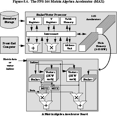
In both dense matrix-matrix multiplication and dense matrix factoring, there are O(n3) floating point operations and O(n2) words of data. It therefore appears possible for a processor to effectively perform O(n) useful floating point operations for every data word referenced from main memory! While the preceding example showed how matrix factoring can achieve a 1:1:1 ratio of fetches to multiplies to adds, it is in fact possible to use m by m block factoring to achieve a ratio of 1:m:m. This led to the development by Floating Point Systems of a special-purpose computer originally called the FPS-164/MAX, which modified the FPS-164 architecture simply by adding arithmetic pipelines, not increasing main memory bandwidth. The effective speed on problems possessing an m by m submatrix structure can be increased by up to 31 times, the maximum number of concurrent multiplier-adders [Charlesworth and Gustafson 86]. Figure 5.4 shows a block diagram of the architecture.
Both matrix multiplication and matrix factoring involve at least O(n2) parallel tasks for n by n dense problems. The parallelism can be exploited to reduce memory bandwidth in two ways:
1. Re-use of data (temporal bandwidth reduction)
2. Broadcast of data (spatial bandwidth reduction)
In multiplying a matrix A times a matrix B, each column in B is used n times; hence the cost of moving a column to a fast local memory is amortized over many clock cycles. Every element in A is eventually applied to a corresponding element in n columns of B, so a broadcast of elements of A to those columns can accomplish useful work. Broadcasting takes the form of multiple processor boards, each mapped to a region of high memory, that can all respond simultaneously to some reserved set of addresses on the memory backplane. Not only does bandwidth reduction unburden the backplane; it also permits the disk storage to keep pace with the arithmetic, which is essential to keep the computer busy for more than a few seconds.
The MAX allows up to 15 extra processor boards, each with two multiply-add pipelines, or 30 pipelines total. The scalar unit of the main processor participates in the column operations using its table memory as a column store, so the actual number of parallel pipelines is 31. Thus, the 11 Mflops pipeline in the FPS-164 can be supplemented to attain a peak of 11 x 31 = 341 Mflops on a highly restricted but very useful set of operations. A single memory reference is used for four multiply-adds per pipeline, so that 248 floating-point operations can be sustained with just one fetch! The full MAX configuration has been successfully used to solve dense linear systems as large as 20000 by 20000 elements in a little over eight hours.
5.6.3 Fourier Transforms
Now consider the problem of evaluating the Discrete Fourier Transform on 64 complex data points. The usual operation count says that evaluating the sum
directly requires O(n2) floating point operations whereas the Fast Fourier Transform (FFT) methods use O(n ln n) operations, a clear improvement. But the sum above is nothing more than a matrix-vector product, where the matrix elements are defined by Wkl = wkl, and that matrix can be re-used for many input functions f(k). Because the MAX can easily do many vector-vector scalar products at once, the architectural parallelism can actually outweigh the algorithmic advantages of the FFT for small numbers of discrete points. The FPS-164, for example, must perform about 2000 floating point operations for a radix-2 FFT on 64 points, requiring over 1300 clock cycles even when highly optimized. The matrix-vector product requires about 16000 floating point operations (multiply-add pairs), but can be done with 16 concurrent complex dot product engines using the MAX, bringing the total time under 500 cycles. For larger Fourier transforms, one can simply build FFT’s out of mixed radices ranging up to radix 64, using matrix-vector methods up to the crossover point and then switching to the factorization methods of the FFT.
This illustrates the flaw of conventional algorithm analysis, which ignores memory references in the work assessment. An FFT must eventually reference every storage location O(ln n) times, and those references cannot all be local; they stride up to halfway across the required storage. The matrix-vector product pays the price of redundant floating-point operations to reduce communication, so that every location of f(k) need only be referenced once! In a hypothetical computer that can compute the parallel inner products with binary sum collapses in O(ln n) time, both methods are ultimately O(ln n) in the time complexity of memory accesses.
5.6.4 Finite Difference Methods
As a final example of algorithm choices affected by the use of compute-intensive architectures, consider the partial differential equations (PDE’s) solved by discretizing time and space and applying a difference operator to approximate the differential operator. A typical case of a two-dimensional problem might resemble the following, in Fortran:
DO 1 I=2,N-1
DO 1 J=2,N-1
1 F(I,J)= U*F(I,J)+V*(F(I-1,J)+F(I+1,J)+F(I,J-1)+F(I,J+1))
where U and V are predefined constants and F(I,J) is a two-dimensional array representing the physical state of the system. For hyperbolic PDE’s, this type of equation might compute the next timestep of the spatial state of the system; for elliptic PDE’s, it might be a relaxation method that produces an F(I,J) that eventually becomes sufficiently close to the solution. In any case, the kernel involves six main memory references and six floating point operations. The memory references are “nearest neighbor” in two dimensions, so the technique of loop unrolling can improve the ratio of arithmetic to memory references:
DO 1 I=2,N-1
DO 1 J=2,N-1,2
F(I,J)=U*F(I,J)+V*(F(I-1,J)+F(I+1,J)+F(I,J-1)+F(I,J+1))
1 F(I,J+1)=U*F(I,J+1)+V*(F(I-1,J+1)+F(I+1,J+1)+F(I,J)+F(I,J+2))
Using registers for expressions that occur more than once, there are 10 memory references and 12 floating point operations. More unrolling allows the ratio to approach 2:3 at the cost of register usage (and possibly exceeding the size of the program cache), which is one argument in favor of a large set of scalar registers. Computers with a 1:1:1 ratio of fetches to multiplies to adds can approach 50% of peak speed with no unrolling, or 66% with extensive unrolling.
An interesting contrast with either of the above methods is the one favored by highly vector-oriented computers. A vector computer might run the problem more efficiently in the following form, where TEMP is a vector register:
DO 10 I=2,N-1
DO 1 J=2,N-1,2
1 TEMP(J)=F(I-1,J)+F(I+1,J)
DO 2 J=2,N-1
2 TEMP(J)=TEMP(J)+F(I,J-1)
DO 3 J=2,N-1
3 TEMP(J)=(TEMP(J)+F(I,J+1))*V
DO 4 J=2,N-1
4 F(I,J)=U*F(I,J)+TEMP(J)
10 CONTINUE
If there is enough bandwidth to either memory or vector registers to keep the floating point functional units busy, and if the vector operations shown are in the repertoire of the hardware that manages the arithmetic, then the preceding method can approach 75% of the peak Mflops rate of machines with one adder and one multiplier functional unit. On the other hand, if TEMP must reside in main memory, then this is a disastrous approach for memory-bound processors. There are twice as many memory references as in the “unvectorized” approaches, causing a multiply-add processor to achieve at most 25% of peak speed. This is why one occasionally observes the phenomenon that the CRAY or CYBER type of processor does relatively better on the vectorized version of an application program, whereas the FPS type of processor does relatively better on the unvectorized version. This is a source of difficulty for the developers of application software, who naturally seek a simple-to-maintain single method that works well on a wide range of compute-intensive machines.
5.7 Metrics for Compute-Intensive Performance
Ultimately, the only performance questions of interest to a computer user are:
1. How long will the application take to run?
2. How much will the run cost?
This assumes, of course, that answers are within required accuracy tolerance. On compute-intensive processors, there is usually a significant hurdle to answering the above questions by direct measurement. Architectures vary greatly, and only considerable conversion effort shows the performance that is ultimately possible. Since compute-intensive processors trade ease-of-use for cost-performance, predicting overall speed and cost (including reprogramming cost amortized over the useful life of the application) is a difficult proposition.
As a result, the industry has come to use simpler metrics that claim correlation with application performance. At the simplest (and most inaccurate) level are machine specification such as clock speed, peak Mflops rating, Mips rating, memory size and speed, disk size and speed, and base system price. An experienced user may find a linear combination of these that correlates well with performance and cost on the application of interest, but these metrics are generally the least useful. Comparisons of clock speeds or Mips are meaningless unless the architectures being compared are practically identical, down to the machine instruction set.
A compromise is to use standard problems that are much simpler than a complete application but exercise a variety of dimensions of machine performance. Compute-intensive processors have their own set of industry-standard benchmarks, of which the following are examples (arranged in rough order of increasing complexity and usefulness at gauging performance):
• Matrix multiplication (no particular size)
• The 1024-point complex FFT.
• Whetstones (a synthetic mixture of operations designed to test scalar speed only).
• Solution of 100 equations in 100 unknowns, with partial pivoting.
• The Livermore Kernels (24 Fortran excerpts from application programs).
• The “four-bit adder” simulation in the SPICE test suite.
• Solving structural analysis problem “SP3” in Swanson’s ANSYS™ test suite.
To compare actual costs, it is similarly possible to estimate total computer cost by considering all hardware costs, software costs, facilities requirements, and conversion effort. The ultimate measure of cost can be determined by the price of the application run at a computer service bureau, which must determine charges accurately enough to remain in business and yet be competitive with alternatives. It is rare for compute-intensive processors to be compared using applications that exercise memory bandwidth or disk speed, for all the reasons stated in the Introduction. This is perhaps unfortunate, since they figure prominently in the performance of applications such as analog circuit simulation and large-scale structural analysis.
5.8 Addendum: Hypercube Computers
Hypercubes [Fox 84, Seitz 84] have emerged as a commercially important class of multicomputers. In contrast with so-called “dance hall” architectures where a set of processors share a set of memories through a switching network, hypercube computers are built out of an ensemble of memory-processor pairs. Each processor-memory “node” is autonomous, and contains communications channels to N other nodes. The channels form the topology of the edges of an N-dimensional cube, which has a number of desirable properties (see Chapter 6).
In practice, at least one channel is used for communication to a host or other I/O device, and the commercial hypercubes have all made this variation on the original prototype built at Caltech in the early 1980’s.
Processors cooperate on a particular task by passing messages explicitly to one another; there is no “shared memory” in the system and hence no need to deal with the problem of multiple writes to a memory location. This latter problem is a major source of indeterminism and programming difficulty in shared memory designs. Both shared memory and hypercube designs pay a cost for global memory accesses that grows logarithmically in the number of processor-memory pairs; the hypercube, however, rewards locality of memory accesses.
Replicated Very Large-Scale Integration (VLSI) is ideal for the nodes of hypercube computers, now that VLSI density has reached the point where a complete processor can fit on a single chip. The early hypercubes use a mixture of small, medium, and large-scale integration to put a node on one or two boards. The implementation by NCUBE, Inc. integrates a complete VAX-style processor with floating point arithmetic, 11 communications channel pairs, and an error-correcting memory interface, on a single chip. With no “glue logic,” this chip plus six memory chips form a complete node with 512 KBytes of memory.
Available hypercubes tend to be either highly compute-intensive or general-purpose. They are largely characterized by three times: communication time, memory-move time, and arithmetic time. The ratio of the last time to the first two determines how compute-intensive the design is.
Communication time is the time to send a message of length n across a single channel. There is a startup time which currently ranges from 18 to 3000 microseconds, followed by transmission at a rate which currently ranges from 1 to 10 microseconds per byte (based on current product literature from Ametek, Intel, NCUBE, and Floating Point Systems). The startup time is largely a function of the amount of protocol used by the software for error detection/correction and for automatic message forwarding to more distant nodes. Low startup times are critical when the application is “fine-grained” and cannot batch together transmitted data into longer structures. This is the communication analog of vector arithmetic.
Memory-move, or “gather-scatter” time, is the time to move data within the memory of a single node. Usually, the communications channels use only a fraction of the memory bus, so moves within a single node are much faster by the reciprocal of that fraction. Currently, time to move a contiguous array from one location to another ranges from 0.1 to 2 microseconds per byte.
Arithmetic time is the time to do a floating point operation (two inputs, one output) by whatever means is provided on the node. For 64-bit operands, the current range is rather wide: from 0.1 to 20 microseconds. The ratio of Arithmetic Time : Communication Time varies from about 1:100 or 1:200 for the FPS T Series or the Intel iPSC/VX, to about 1:1 for the NCUBE. The T Series and iPSC/VX are extremely compute-intensive and use vector arithmetic managed by a microprocessor, whereas the NCUBE uses integrated scalar arithmetic.
The arguments of earlier sections regarding system balance apply here, with the added consideration of “surface area.” Ideally, each node communicates and computes at the same time, and sees no bottleneck from either activity. On the T Series or the iPSC/VX, every word brought over a channel must participate in over 100 floating point operations if the arithmetic is to be kept busy. Suppose that the application is the Synthetic Seismic problem, modeling the wave equation in three dimensions. Each grid point requires eight floating-point operations per timestep in the simplest acoustic model. When the three-dimensional domain of the problem is partitioned into n by n by n subdomains, one per processor, there will be 6n2 points on the “surface” and n3 points on the “interior” of the node memory. Each timestep will require the exchange of 6n2 words of data (both in and out) and will perform 8n3 floating point operations, a ratio of 4/3n. For optimum balance, this number should approximate the Communication Time : Arithmetic Time ratio. If this ratio is 100:1, then the two timesteps in each node will require 2 million words, or 16 million bytes, per node just for the data!
This illustrates a growing problem in computer design: memory technology lags floating point arithmetic technology by two years or more, so users must await fourfold or sixteenfold increases in commodity memory chip densities before the announced compute-intensive ensembles reach the minimum main storage needed for reasonable system balance. The advent of floating point chip sets such as those made by AMD and Weitek have made it easy to add several Mflops of peak performance to an ordinary microprocessor. Everyone who does so soon notices that a 10 Mflops 64-bit engine unfortunately consumes 240 MBytes/second and at least 10 Mips for effective control. This brings to the fore all the issues discussed in previous sections… methods such as a large register set for reducing bandwidth, and vector instructions in microcode for reducing required Mips. For high Mflops rates which do not compromise on bandwidth or control, the simplest solution is to have more nodes as in the NCUBE processor, highly integrated so that many nodes can be reliably put into a small space with small power requirements. The 500 Mflops rating of the 1024-node NCUBE is similar to that of the compute-intensive hypercubes, but very dissimilar in that those 500 Mflops are accompanied with 10 GBytes of bandwidth and over 2000 Mips of control; its node memory is capacious relative to the amount required for compute/communicate balance.
5.9 Concluding Comments
In the spectrum of computer architectures, compute-intensive designs may indicate the future of all designs. As switching devices become ever faster and cheaper relative to the wires that send the information, all computers may ultimately be able to regard arithmetic operations as free relative to the cost of moving data. The traditional measures of algorithmic work using floating point operation counts may soon be just as misleading on general-purpose computers as they are on compute-intensive ones, as computer designers push closer to the physical limits imposed on the speed that information can travel.
The feature that will remain distinctive of compute-intensive designs is that they trade ease-of-use, interactivity, and generality for cost-performance. They are neither “inferior” nor “superior” to general-purpose computers; they simply have a different feature emphasis. The availability of computers that make this tradeoff will continue to bring large-scale scientific applications within the reach of users who would otherwise not be able to afford to do them.
Acknowledgements
The author obtained much of the information in this chapter while working on applications at Floating Point Systems, Inc. That experience was invaluable in providing a cross-section of both compute-intensive architectures and compute-intensive applications of both academic and commercial importance. Alan Charlesworth, Staff Engineer at FPS, is in particular due much thanks for many hours of insightful discussion.
#