Figure 1. Matrix-vector product forms.
by
Floating Point Systems, Inc.
Large-scale scientific computing is dominated by the "crunching of numbers." By performing billions of multiplies and adds on millions of simulated data points, scientists can model physical phenomena, like the flow of air around a supersonic airplane or the movement of storms in the atmosphere. The data values range over more than fifty orders of magnitude, from the inside of a quark to the circumference of the universe. Because a simulation sun is made up of thousands of iterated computation steps, at least eight significant digits must be retained by each arithmetic operation to avoid excessive round-off errors in the results.
The 16- and 32-bit integer arithmetic common in business computing does not provide adequate range or accuracy for scientific use. Instead, scientific applications normally use 64-bit floating-point arithmetic. IEEE standard double-precision arithmetic,1 for example, provides a dynamic range of 616 orders of magnitude and a precision of 15 significant digits. Because arithmetic speed usually dominates overall execution times, the performance of scientific computers is traditionally measured in MFLOPS, or millions of floating-point operations per second. Current processor implementations range from a speed of one-twentieth MFLOP for the best personal computer CPU to several hundred MFLOP' per supercomputer CPU.
Unfortunately, the automata scaling and wide word widths of floating-point arithmetic operations are quite complicated.2 For example, the implementation of a fast 32-bit integer adder requires approximately 1200 two-input gates, while a fast 64-bit floating point adder needs about 13,000 gates. Before the advent of VLSI (over 10,000 gates per chip), it was very expensive to implement this amount of logic. The data unit (adder, multiplier, registers, and interconnect buses) of the 11-MFLOP FPS-164 Scientific Computer, designed in 1979 with medium-scale integration (10 to 100 gates per chip), required nearly 2000 chips. It occupied seven large (16- x 22-inch) printed circuit boards and dissipated 760 watts of power (see Table 1). This sizable amount of hardware made it rare for a CPU to have more than one set of floating-point arithmetic.
| Table 1 | |||
|---|---|---|---|
| The impact of VLSI on number-crunching. | |||
| Technology | |||
| Functional Unit | 1979 MSI | 1985 VLSI | Improvement |
| Data unit (10-20 MFLOP arithmetic, registers, and interconnecton buses) | 2450 sq.in. 760 watts | 39 sq.in. 18 watts | 63x 42x |
| Control unit (program and data memory address generation) | 700 sq.in. 240 watts | 6 sq.in. 4 watts | 116x 60x |
| Memory (250 ns cycle, 1 million 64-bit words) | 5600 sq.in. 430 watts | 350 sq.in. 40 watts | 16x 11x |
The business of implementing high-speed scientific computing was forever altered in mid-1984, when Weitek, Inc., of Sunnyvale, California announced the first commercial leap from MSI to VLSI for fast 64-bit arithmetic.3 This advance reduced the size of a high-speed floating-point data unit from several thousand chips to nine chips. For the first time it was possible to greatly improve performance by including many sets of arithmetic in a CPU. The FPS-164/MAX Scientific Computer, initially delivered in April 1985, is the first computer to be implemented from replicated VLSI arithmetic p arts--and the first computer to provide several hundred MFLOPs in a supermini-priced processor.
By mid-1985, two MOS VLSI number-crunching chip sets had been publicly announced, 4.5 and several others were in development. They provide a reasonably complete selection of CPU functions (see Table 2). By the time commercial 1.25-micron parts appear in late 1986, it is reasonable to expect a two-chip CPU set (data unit chip/control unit chip). With this plethora of new VLSI parts, the opportunities for VLSI-based scientific computing are almost unbounded. The fifty-fold improvement attained so far by these VLSI parts over their MSI equivalents challenges today's computer architect to achieve one gigaflop in the same sevenboard space where only 10 MFLOPs fit in 1979.
| Table 2 | ||||
|---|---|---|---|---|
| Announced MOS VLSI number-crunching parts as of mid-1985. | ||||
| Function | Part | Max. | Throughput | Technology | Floating-point multiplier | WTL 1264 | 8 MFLOPs 4 MFLOPs | 32 bits 64 bits | NMOS |
| ADSP-3210 | 10 MFLOPs 2.5 MFLOPs | 32 bits 64 bits | CMOS | |
| Floating-point ALU | WTL 1265 ADSP-3220 | 8 MFLOPs 10 MFLOPs | 32 & 64 bits 32 & 64 bits | NMOS CMOS |
| Register reservation unit | WTL 2068 | 8-12.5 Mhz | CMOS | |
| Integer ALU | Two ADSP-1201s WTL 2067 | 10 Mhz 8-12.5 Mhz | CMOS CMOS |
|
| Multiport register file | WTL 1066 | 8 Mhz | NMOS | |
| Memory address generator | ADSP-1410 | 10 Mhz | CMOS | |
| Program sequencer | ADSP-1401 WTL 2069 | 10 Mhz 8-12.5 Mhz | CMOS CMOS |
|
| 256K static column DRAM | I51C256H | 15 Mhz | CMOS | |
| Abbreviations: WTL=Weitek Corp.; ADSP=Analog Devices, Inc.; I=Intel Corp. | ||||
MOS VLSI number-crunching components have by far the lowest power dissipation per MFLOP of any implementation option and hence are the most cost-effective way to implement high-speed scientific computing. The speed of a single MOS chip set is limited by internal gate delays to around 20 MFLOPs. Von Neumann computers (whether IBM PC or Cray) do only one operation at a time and hence can usefully employ only one set of arithmetic hardware (VLSI or otherwise) per CPU. Thus the performance of such a CPU implemented with MOS VLSI parts is limited to roughly 20 MFLOPs, which is adequate for much useful work but not for supercomputing. There are two options: to build monolithic processors out of very fast but very hot and expensive low-integration components (such as emitter-coupled logic or gallium arsenide) or to build a parallel processing system out of multiple MOS VLSI chip sets.
At 20 MFLOPs per CPU chip set, it takes only a 50-processor system to reach a total of one gigaflop. For such a system to be useful, though, algorithms must have enough potential concurrency to effectively employ at least this many processors. Fortunately, recent research at Caltech suggests that many problems have sufficient potential parallelism to utilize 10,000 to 100,000 concurrent computing nodes.6 The strategy is to divide the universe being simulated into subdomains that are allocated one per processing node. Each node computes upon its particular volume and communicates the relevant boundary information to its neighbors. Since volume grows faster than surface area, the communication rate required between nodes can be traded off against the amount of memory required per processing node by increasing the computational volume handled by each node. The division of the problem space among the processors is done explicitly by the applications designer, and communication is accomplished via message-passing software cells.
As each new generation of improved VLSI technology drives down the cost of processors and memory, the expense of communication (such as board wiring space, cables, and connectors) can dominate.7 This pitfall can be avoided by implementing systems with only the minimum amount of internodal communication required to solve the dominant problem of interest (see Table 3).
| Table 3 | |||
|---|---|---|---|
| Hierarchy of multiprocessor connectivity | |||
| Topology | Number of Communication Ports/Node | Maximum Concurrent Data Transfers | Example Applications |
| Bus | 1 | 1 | Time-sharing replacement |
| Broadcast bus | 1 | n | Matrix multiply-factoring |
| m-dimension mesh | 2m | 2nm | Signal processing, matrix arithmetic |
| Logarithmic (hypercube) Crossbar | 2log2n 2n2 | 2log2n 2n3 | FFT, circuit simulation Shared memory |
| Note: n=number of processing nodes | |||
A bus interconnect has only a single communications port per processing node but can correspondingly accommodate only a single transfer per unit time. This bottleneck limits the degree of parallelism to at most a few dozen nodes (see, for example, the Encore system8). A broadcast bus can send a single data item to all bus destinations in a unit time. This is the minimum amount of connectivity required to perform matrix multiplication and factoring with up to several hundred logically parallel nodes; thus the broadcast bus is the interconnect of choice for the FPS-164/MAX matrix supercomputer.
In a mesh of nodes, each processor can simultaneously send to or receive from its nearest neighbors along each dimension of the mesh at a cost of two communications ports per dimension. The size of the mesh can be extended indefinitely, but doing so also indefinitely extends the distance between arbitrary nodes. Meshes are best for algorithms where the data can flow locally, stop by step across the system, as in a macroscopic pipeline. The CMU Systolic Array Computer9 is an example of a one-dimensional mesh intended for signal and image processing.
In a logarithmic interconnect, such as a Boolean hypercube, the number of ports per node grows with the logarithm of the number of nodes. This means that the distance between arbitrary nodes also grows only logarithmically, which is necessary for problems with significant nonlocal communication, such as the FFT. The Caltech Cosmic Cube is a demonstration six-dimensional hypercube using 0.05 MFLOP nodes based on the Intel 8086/8087.10 Intel has recently marketed a version of this system called the Personal SuperComputer (iPSC).11 Finally, in a crossbar connection each node is connected to every other. This scheme is feasible only for systems using a small number of nodes, such as the 16-processor C.mmp,12 and has been historically used to implement multiport shared memories for mainframe systems.
The problems of engineering and applied physics can be classified into two broad categories: lumped systems ad distributed systems. Lumped systems, such as mechanics and electric circuit theory, have only one independent variable: time; hence they are described by ordinary differential equations. Distributed systems, or fields, model spatial dimensions as well as time. The concept of continuous fields has wide-ranging applications throughout physics and engineering, including such diverse areas as heat transfer, fluid mechanics, electrostatics, electromagnetics, acoustics, and particle diffusion.13
A continuous field is approximated by segmenting it into a mesh of node points and then discretizing the differential equations that describe the field to produce local element matrices for each node. These local matrices are assembled into a global system matrix by superposition. Finally, the global matrix, representing a system of simultaneous linear equations, is solved for the unknown variables, such as pressure or temperature. For nonlinear or time-dependent problems, the entire process must be repeated many times for every deformation increment, or time slice.14
To improve the resolution of the model, the number of node elements can be increased, or a finer time step used. Either method drastically increases the computation time. For large problems, the global solution step is dominant, and hence there is demand for faster solution of larger matrices. Fortunately, it is an excellent application for a replicated VLSI architecture.
Matrix-vector product. The MVP is the simple but fundamental operation that dominates scientific matrix computing.15 It is the basis of both matrix multiplication and linear equation solving and is the primary operation around which all supercomputers are designed and benchmarked.16
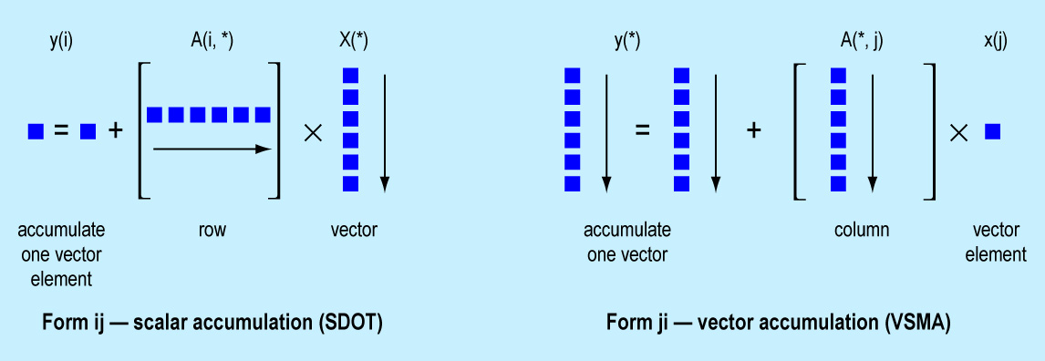
Product forms. The MVP is a sum-of-products operation: y = A * x, where y is a vector with m elements, A is a matrix with m rows and n columns, and x is a vector with n elements. In Fortran, this may be expressed as either of the following doubly nested loops, which differ only in the order of loop nesting:15
Form ij--scalar accumulation (SDOT)
    DO 20 i = 1, m
         y(i) = 0.0
         DO 30 j = 1, n
              y(i) = y(i) + A(i,j) * x(j)
30     CONTINUE
20  CONTINUE


Form ji--vector accumulation (SAXPY)

    Do 10 i = 1, m
            y(i) = 0.0
10  CONTINUE
    DO 20 j = 1, n
         DO 30 i = 1, m
              y(i) = y(i) + A(i,j) * x(j)
30    CONTINUE
20  CONTINUE
Note that the computation performed by the two forms is identical: the accumulation in y of a row or column of A multiplied by x. Both forms yield the same answers, including round-off errors, and both require the same amount of arithmetic work.
Figure 1. Matrix-vector product forms.
Locality of accumulation. The difference between these two forms is in the locality of the accumulation (Figure 1). form ij accumulates into a single element of y the sum of the element-by-element products of a row of y against the vector x. This is termed in mathematics a dot product, and is the SDOT routine in the widely used Basic Linear Algebra Subprogram (BLAS) library.17 The complete MVP is accomplished by m dot products, involving the same vector x with successive rows of A. Form ji, on the other hand, accumulates into all the elements of y the products of a single element of x with the respective element of a column of A. It is the SAXPY (for "A times X Plus Y") routine of the BLAS. Below, it is called VSMA, for vector/scalar multiply-add. A complete MVP is accomplished by n such VSMA operations, involving successive elements of x against successive columns of A.
Cost of accumulations. The locality of the summation is critical to implementation costs, since y must be both read and written for each accumulation, while A and x are only read. Thus the access rate required of y is double that of A and x. The SDOT form sums a scalar (single element) at a time, which means that a high-speed register can be used to hold the single element of y being accumulated. The VSMA form, on the other hand, sums across an entire vector, requiring a several-thousand-word memory (64 bits wide) to hold all of y. Two copies of this vector memory will usually be required: one to supply read data and one to accept writes of updated accumulations. Thus, at a given performance level, the VSMA form will be more expensive than the SDOT form. Or, if only one y vector register can be used per multiply-adder, then VSMA will run at half the rate of SDOT.
A possible countervailing factor may occur of a pipelined adder is used. A pipeline is like a bucket brigade at a fire. Many buckets can be in transit to the fire at any instant in time; likewise several sums can be in process of completion at once. Thus, when SDOT is used, there will be as many partial sums being accumulated in the adder as there are stages (S) in the adder pipeline: two to eight is a typical number. At the completion of the dot product, the partial sums in the pipeline have to be collapsed into a single sum before being stored into y. The overhead is approximately S(log2( S) + 1) arithmetic cycles. For eight stages, this is 32 cycles, which would be a serious (100%) overhead if the dimensions were as small as 32. For larger dimensions (like 1000) the overhead dwindles to insignificance (3%). The other way around this problem is to accumulate S different dot products simultaneously, one is each stage of the adder. Note that VSMA doesn't have a problem using pipelined arithmetic, provided that the problem dimensions are greater than S.
Parallel matrix-vector products. If scientific matrix problems required only a single matrix-vector product at a time, the only way to increase speed would be to use faster arithmetic and memory circuits to implement a monolithic MVP unit. Indeed, this rationale has driven designers of current supercomputers to use the fastest available ECL bipolar technologies. Fortunately, however, problems involving matrix-vector products always require multiple MVPs to be evaluated. In a matrix multiply or factor, there are on the order of n different x vectors that all need to be multiplied by the same matrix A (where n is the dimension of the matrix). Thus, an alternative tactic for gaining speed is to devise parallel versions of the matrix-vector product. Then, the most cost-effective technology can be used to implement an MVP module. The speed of a single module is not critical, since overall performance can be attained by replication.
Parallel forms. The minimum resources required to implement a replicatable MVP module are a 64-bit floating-point multiply-adder, a scalar register to hold a single element of x and a vector register to hold the elements of y. Externally, a memory is needed to hold A, along with a connection over which a stream of successive Aij row elements can be broadcast to all the modules (Figure 2).
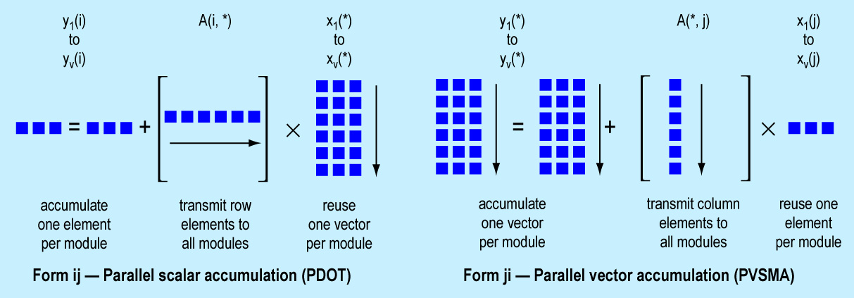
Figure 2. Parallel matrix-vector product forms.
For a parallel scalar accumulation (PDOT), each of v modules receives a broadcast row element of A, multiplies it by the corresponding element of x from its own vector register, and sums the resulting element of y into its own scalar register. For a parallel vector accumulation (PVSMA), each module multiplies a broadcast column element of A by the element of x from its own scalar register, and sums that into the appropriate element of y from its own vector register. Assuming that the minimum of one vector register is provided per module, then PVSMA will operate at half the speed of PDOT.
Parallel implementations. Because only a moderate number of modules are involved, the elements of A can be broadcast to the modules across a conventional bus. The bus must be able to transmit a 64-bit value every multiply-add time-step. At 6 MHz, for example, this is a 48 Mbytes/second communication rate. The rate can be reduced if room is provided to hold several vectors in each module. The module can do several multiply-adds with each broadcast data value. For example, if a module can hold four vectors, the communication rate for A can be reduced to one quarter, or 12 Mbytes/second at a 6 MHz clock. In this manner, the size of the local vector storage in each module can be traded off against communication bandwidth, so that, if desired, a board-level MVP module can be scaled down to fit within the constraints of a standard bus (e.g., Multibus II or VMEbus).
Soon it will be possible to fit the floating-point arithmetic, control, and communications interface on an MVP module onto two VLSI chips, eliminating the power and space consumed by the MSI "glue" logic required in an off-the-shelf design. Then, an entire module would consist of only the two processing chips, plus one to four 256K dynamic RAMs for vector storage. Given 10 MFLOPs (and 2 watts) per chip-scale module, total performance of one gigaflop will be possible from only a few hundred chips dissipating a few hundred watts. Because of the number of modules and the limited drive capability of VLSI chips, it will not be appropriate to use broadcast communication. Instead, a one-dimensional systolic pipeline can be arranged to feed data directly between adjacent chips.9
The FPS-164/MAX matrix supercomputer is the combination of a low-cost scientific computer with up to 15 VLSI-based matrix-vector product board-modules (Figure 3).
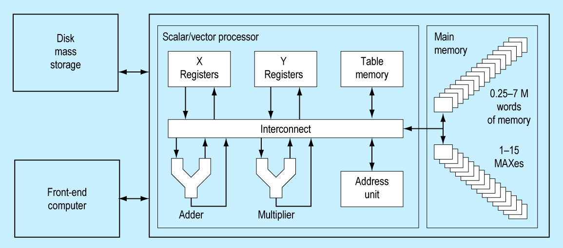
Figure 3. FPS-164/MAX Scientific Computer.
Since each physical module implements eight logical modules, the maximum parallelism is of the order 120. The FPS-164 provides the considerable system resources necessary for large-scale scientific computing.18 These include 11 MFLOPs of 64-bit floating-point vector and scalar arithmetic, a large physical memory (up to 15 megawords), an optimizing Fortran-77 compiler, and a capacious disk storage (up to 17.3 billion words). It is used both as a Fortran-programmable scientific mainframe and as a dedicated computer to run engineering packages, such as Ansys (for structural analysis) or Spice (for electrical circuit simulation). For a more detailed description of the MAX module see Madura et al.19
The FPS-164/MAX, like many supercomputers, is always networked with a mainframe or superminicomputer, such as a VAX-11/780, and IBM 4XXX, or an IBM 30XX. The front-end computer handles interactive time-sharing, while the FPS-164/MAX concentrates on arithmetic-intensive calculations. This division of labor allows each computer to be used more cost effectively and avoids the need to change the entire computing environment to accommodate the increasing demands of scientific computing.
MAX module architecture. Just as the FPS-164 enhances an interactive mainframe for general scientific computing, the Matrix Algebra Xcelerator (MAX) modules enhance the FPS-164 CPU for linear algebra. The module architecture is tuned exclusively for the matrix-vector product. Because the FPS-164 can supply a large memory and general Fortran programmability and because the MVP is such a very regular operation, it has been possible to minimize the amount of memory, control, and communications support logic required per module, in favor of maximizing the amount of VLSI floating-point arithmetic.
Communication. The parallel matrix-vector product A*x is performed by broadcasting data from A to all the replicated modules, each of which holds a different vector x. The total number of data points required per floating-point operation is very low, on the order of 1/n for an n x n matrix, so that a very high aggregate performance can be supported with a moderate bus rate. The FPS-164 memory subsystem, with a synchronous memory bus (to permit broadcasting), no data cache (to avoid stale data problems), and up to 29 large (16- x 22-inch) board slots available, is an ideal existing physical framework for board-scale replication. Each MAX module is implemented as a storage board that plugs into an FPS-164 memory slot.
The FPS-164/MAX has a 16-megaword address space, of which 15 megawords can be used to address physical memory. The highest megaword of the address space is divided into 16 64K-word segments, one for each of up to 15 MAX modules (Figure 4).
Figure 4. FPS-164/MAX memory map.
The last 64K address segment is the broadcast segment, which is recognized by all the modules so that data or control can be director simultaneously to all 15 modules. Inside a particular module, the lower 32K addresses are divided into eight 4K-word blocks, one for each vector register. Finally, each module has several addresses for its scalar status, and control registers and for supplying data to initiate computing. A program writes data into or reads results from a MAX module by the same two-instruction copy loop used to move data between other portions of FPS-164 memory. The modules are, in effect, very smart memory for the FPS-164 CPU, since they have both computational ability and storage.
Control. The matrix-vector product is a very orderly operation. A stream of matrix elements is broadcast to each module, which does a multiply-add with data contained locally. Since all modules perform the same computational sequence in lock-step, this is single instruction/multiple data (SIMD) control, the simplest form of parallel architecture. Essentially no control needs to be replicated in each module.
There is no program sequencing inside the MAX modules; instead, a program inside the FPS-164 CPU synchronously directs operation of each module by writing to the various MAX control addresses within a given 64K address segment (Figure 4). Or it can control all modules simultaneously by using the Broadcast segment. Writing to the Control Register address selects the vector form for the next computation. The VectorRegisterIndex address sets the next location in the vector registers to be operated on. Writing data to the AdvancePipe address actually causes a multiply-add to take place. As an option, IncrementIndex, which will post-increment the VectorRegisterIndex, can also be chosen. Finally, an optional Collapse can be chosen, to complete the summation of the partial products in a pipelined PDOT operation.
In operation, the FPS-164 program selects the vector form in al the modules by writing to the ControlRegister address in the Broadcast address segment. Next, it writes to the Broadcast segment's VectorRegisterIndex address to set the starting address for all the MAX modules. Then, after copying different matrix rows into each vector register, the program loops, reading a matrix column element from FPS-164 memory and writing it to the Broadcast segment's AdvancePipe & IncrementIndex address. This sequence causes all modules to do a multiply-add and advance to the next vector register element. Usually, the same program loop that directs computing in the MAX can also route data to the FPS-164 CPU's own multiplier and adder, so the CPU's compute performance need not be wasted.
Memory. The total amount of memory required for operations on matrices may be quite large. A modest 1K x 1K matrix, when fully populated, occupies one megaword. If each replicated module required this much memory, the storage cost would be unbearable. For tunately, for n x n matrices, only O(Ãn) storage is required per module--enough to hold a few vectors.
The MAX modules can directly accommodate up to 2K long vectors, corresponding to a four-megaword, full matrix. Larger sized are handled by operating on multiple 2K-element subvectors. An additional 2K words of address space per vector and scalar register to feed each of its two space to permit every broadcast matrix element to be computed against four vectors per multiply-adder. The 4:1 local reuse is necessary to avoid using up 100 percent of the FPS-164 memory system's bandwidth. A four-instruction loop, with only two memory operations, leaves 50 percent of the memory bandwidth for disk I/O or for supplying vector register indices for sparse-matrix addressing techniques.
Arithmetic. In a matrix-vector product the multiply is always followed by an add, so the VLSI arithmetic chips in the MAX modules are hardwired into this pattern (Figure 5).
Figure 5. MAX matrix-vector product module.
The data element written to the AdvancePipe address is always one of the multiplier operands, and the multiplier always feeds the adder. The only data path choices, then, are the connections of the vector and scalar registers, which may be used to do a scalar accumulation (PDOT), vector accumulation (PVSMA), or vector multiply-scalar add (PVMSA) (see Table 4).
| Table 4 | ||
|---|---|---|
| MAX vector forms | ||
| Name | Operation | Speed per MAX Module |
| Parallel scalar accumulation (PDOT) | S0 - 7<--A * Vi0 - 7 + S0 - 7 | 22 MFLOPs |
| Parallel vector accumulation | ||
| (PVSMA1) | Vi4-7<--A*S0 - 3 + Vi0 - 3 | 11 MFLOPs |
| (PVMSA2) | Vi0-3<--A*S0 - 3 + Vi4 - 7 | 11 MFLOPs |
| Parallel vector multiply/scalar add | ||
| (PVSMA1) | Vi4-7<--A*V0 - 3 + Si0 - 3 | 11 MFLOPs |
| (PVSMA1) | Vi0 - 3<--A*S4 - 7 + Vi0 - 3 | 11 MFLOPs |
| A = Data written to AdvancePipe address Sn - m= Scalar registers n through m. Vn - m= Vector registers n through m Vi= VectorRegisterIndex (may be autoincremented) |
||
| Note: Data may be type real or complex. | ||
For every multiply-add, the PDOT form requires only a single read of the vector registers, as well as a read/write of the scalar registers (which, being much smaller, can be designed to be twice as fast). Thus in this form the two sets of vector registers can keep the two multiply-adders fully occupied, producing a maximum of 22 MFLOPs per MAX module, for a possible overall maximum of 341 MFLOPs (including the FPS-164's own arithmetic). The PVSMA form requires twice as much vector register bandwidth and so can support only one multiply-adder, for 11 MFLOPs per module, or 170 MFLOPs total.
With a suitable arrangement of data in the vector registers, the MAX modules can perform either real or complex arithmetic operations at the same MFLOP rate. Naturally, since a complex multiply-add has four times as many operations as the real form, a complex operation takes four times as long to complete as the same-dimension real operation. If the AdvancePipe & AutoIncrement addresses are used to trigger computing in the modules, successive locations are used in the vector registers, as is appropriate for full, banded, or profile matrices. If, however, the VectorRegisterIndex is set before each multiply-add, indirect-addressing techniques can be used for operating on random sparse matrices. In this case, the program reads the indices from a table of pointers in FPS-164 memory. The resulting four-instruction compute loop operates at nearly the same efficiency as the full matrix case, degraded only by I/O memory contention.
MAX software. The MAX modules can be accessed by four levels of FPS-164 software, depending upon the needs of the user for progressively more detailed control of the computation. This modular approach encourages software portability by localizing the interface between the relatively invariant algorithm and the transitory hardware. These standardized software interfaces cover a range of hard configurations, with and without MAX modules, transparently to the global applications program.
Applications packages. These perform a complete end-user solution for an engineering discipline like structural analysis. They are appropriate for the user who perceives the FPS-164/MAX as a tool, not as a computer. ABAQUS, a finite-element package from Hibbet, Karlsonn, Sorenson, makes use of MAX for matrix solutions.
Standard linear algebra software. The Fast Matrix Solution Library (FMSLIB) provides a complete set of equation-solving routines for use by an applications package designer. It efficiently solves real or complex, symmetric or nonsymmetric, simultaneous linear equations for problems so large as to require "out of core" techniques. It is applicable to a wide range of problems, from finite element analysis to electromagnetic boundary value problems. FMSLIB will run at near full efficiency on configurations ranging from none to 15 MAX modules, with varying amounts of FPS-164 memory for buffering submatrices.
Fortran call library. This set of subroutines allows a Fortran program to load submatrices into the MAX modules, to initiate parallel operations such as dot product or VSMA computations, and to read back results. In a typical scientific computation, 5 percent of the code will perform at least 95 percent of the work. When this work involves matrix computations, then it is appropriate to convert this 5 percent of the code into MAX subroutine library calls.
Assembly language. Directly accessing the MAX modules involves writing in the multiparcel, pipelined assembly language of the FPS-164. The code itself is rather simple, consisting mostly of memory-to-memory love loops, which load data into the MAX vector registers or sequence through parallel dot products or VSMAs.
A fundamental operation in linear algebra is the process of multiplying two matrices together. The process is conceptually simple, but the total number of floating-point operations is quite large: n3 multiply-adds, where n is the dimension of the matrix. In comparison, the somewhat more complicated algorithms for solving a system of linear equations (1/3n3 multiply-adds) or QR factorization of a matrix (2/3n3 multiply-adds), actually require less work. The use of MAX is similar in all these algorithms so in the following examples matrix multiplication is used for the simplest illustration.
Sequential matrix multiplication. We wish to compute the product C = A * B, where A, B, and C are n x n matrices of real numbers.
(gif)
In vector terms, to find the ijth entry in C, one takes the dot product of row i in A with column j in B. Unequal dimensions and complex elements are handled by straightforward extensions to this algorithm. A translation into sequential Fortran looks like this triply nested loop:
       DO 10 I = 1, n
            DO 20 j = 1, n
               C(i, j) = 0.0
               DO 30 k = 1, n
                  C(i, j) = C(i, j) + A(i, k) * B(k, j)
30           CONTINUE
20        CONTINUE
10     CONTINUE
Parallel matrix multiplication forms.
The above code is but one of the six possible loop permutations for the matrix multiply, depending upon the ordering of the i, j and k loops.14 In each case a parallel version is made by distributing v iterations of the outer loop into v modules, where v is no greater than n. A parallel version of the inner loop is computed (see Figure 6).
Figure 6. Parallel matrix multiplication forms.
These six versions are identical except for the locality of accumulation, which will have a major effect on performance, depending upon the parallel architecture.
In parallel scalar accumulation (forms ijk and jik), the v modules each accumulate O(1) result at a time. This is the PDOT form of the parallel matrix-vector product, which MAX modules can execute at near their maximum rate of 22 MFLOPs each. In parallel vector accumulation (forms ikj and jki), the v modules each accumulate O(n) results at a time. This is the PVSMA form of the matrix-vector product, which MAX modules can execute at half their maximum rate.
In parallel matrix accumulation (forms kij and kji), the v modules each simultaneously update the partial sum that is a single element of C when complete, requiring a matrix memory that can simultaneously perform v reads and v writes to the same memory location. This is far too much bandwidth to handle with the simple broadcast-based communications used for MAX. A floating-point version of the replace-add operation proposed for the NYU Ultracomputer20 could accomplish this feat. It uses a multistage switching network to collapse multiple adds directed at the same memory location. A more obvious possibility is to use O(n2) processors, in which case each can do its accumulation locally.21 As one may surmise, locality of reference is the dominant consideration in parallel execution.
Within each locality of accumulation, the differences are in the row and column ordering. In the first form of each pair, C is accumulated by row, and in the second form C is accumulated by column. On supercomputers with highly interleaved memories, the ordering may dominate the choice of form. Since feeding the MAX modules requires no more bandwidth than can be supplied by any one FPS-164 memory bank, the choice of ordering is not a critical matter.
Parallel matrix multiplication using the FPS-164/MAX.
Form ijk of matrix multiplication is done by performing v iterations of the outer (i) loop simultaneously in multiple MAX modules, where v is less than or equal to n. Since each row of A is reused n times in the j loop, a total of v of these loops can be distributed into the vector registers of the MAX modules and into the table memory of the FPS-164. Then the j iterations of the inner (k) loop can be calculated by the parallel dot product (PDOT) form of the matrix-vector product (Figure 7).
Figure 7. Parallel matrix multiply on the FPS-164/MAX.
This is expressed in Fortran as:
    p = 2*m+1
    v = 4*p
    DO 10 i = 1, n - v + 1, v
      CALL PLOAD(A(i, 1), n, 1, n, v)
      DO 20 j = 1, n
         CALL PDOT(B(1, j), 1, n, C(i, j), 1, v)
20        CONTINUE
10  CONTINUE
where PLOAD and PDOT are assembly language subroutines from the MAX support library.
This program fragment is explained line by line as follows:
There are two multiply-add pipelines in each of m MAX modules, plus one in the FPS-164 CPU. So, given a full complement of 15 MAX modules, the maximum number of arithmetic pipelines (p) is 31, for an asymptotic 31-fold speed-up over the FPS-164 scalar processor.
Each of the p pipelines operates on four vectors in round-round fashion, so that, given a full complement of 15 MAX modules the matrix is processed in increments of 124 vectors (v) per loop iteration.
The i-loop steps through matrices A and C in blocks of v rows at a time. It thus takes n/v iterations of the i-loop to complete the multiply.
Parameters for PLOAD:
                           A(1, 1)  = initial row element of A to load into the modules
                                n   = stride between row elements of A
                                1   = stride between successive rows of A
                                n   = row length of A
                                v   = number of vectors to load
PLOAD loads eight successive rows of A into the vector registers of each MAX module, plus four rows into the table memory of the FPS-164. The stride between elements in a given row is n because Fortran stores matrices in column order.
The parallel dot product is done n times, once for each column in B. This is a total on n * v dot products per loading of rows into the MAX modules.
Parameters for PDOT:
                        B(1, j) = initial column element of B to broadcast to the modules
                              1 = stride between column elements of B
                              n = column length of B
                       C(i, j)  = initial column element of C
                              1 = stride between column elements of C
                              v = number of parallel dot products
PDOT clears the v scalar registers and then does an n element dot product of the jth column of B against all the v rows of A that are resident in the MAX modules and in the FPS-164 table memory. At the completion of the parallel dot product, the v result elements are stored into the jth column of C.
The two loops take n2/v iterations instead of n2. The timing components are summarized in Table 5.
| Table 5 | |
|---|---|
| Matrix multiply timing | |
| Cycles | |
| Work | |
| Multiply-adds | 4n3/v (v=4, 12, 20, . . . 124) |
| Overheads | |
| Fortran subroutine calls | ~100(n2 + n)/v |
| Vector loads into modules | 2n2 |
| Result reads from modules | 2n2 |
| Pipeline start-up and dot product collapse | 26n2/v |
The speedup approaches p (which is v/4, or 2m + 1) when n>>v and n>>0. Figure 8 shows overall performance on matrix multiply, and Figure 9 shows efficiency, defined as the realized fraction of peak performance (22 MFLOPs/module). The "stair steps" are caused by quantization effects that occur when n is just a little larger than an even multiple of v. In such a case, only a few of the modules (n modulo v) will be doing useful work during the last i-loop iteration. For large n(like 2048), the curves smooth out, since v is at most 124 and hence much less than n.
Figure 8. Matrix multiplication performance.
Figure 9. Matrix multiplication efficiency.
To multiply very large matrices stored on disk, one sues a familiar double-buffering scheme to overlap I/O and computing. The previous submatrix result is written to the disk, and the next operands are read from the disk, all during computation of the current matrix product. Since each point in an n x nsubmatrix is used O(n) times, the disk can keep up with the arithmetic for any reasonable-sized submatrix, say 50x50. One simply codes buffering loops around the above example and uses the DOE extensions to Fortran-77, which allow disk I/O to occur simultaneously and asynchronously during computation.
Solving linear equations. If one replaces the kernel of matrix multiplication by
where L and U are lower triangular and upper triangular matrices, one has essentially the code needed to solve systems of n equations in n unknowns. The MAX architecture applies to solving systems of equations as well as to matrix multiplication. The methods of dealing with disk-resident problems by using active submatrices work equally well here. Factorization required that the computed dot products be used directly to update the submatrix elements, a feature incorporated into the MAX design.
Function evaluation. As an example of a less obvious use of the parallel multiply-add architecture, consider the problem of evaluating intrinsic functions like SIN, EXP, and ATN with polynomial approximations. A polynomial can be thought of as the dot product of a vector (1, x,x2, ..., xn) with a vector of coefficients. If one wishes to evaluate several polynomial functions Pi of several unknowns xj, the evaluation is equivalent to a matrix multiplication. The matrix of powers of the xj elements can be computed during the matrix multiplication. Therefore the MAX is not restricted to equation solving but can also participate in kernel operations associated with equation setup.
The actual use of such specialized hardware in particular applications is best shown by examples. The following three application areas illustrate increasing emphasis on matrix algebra as a percentage of the total run.
Structural analysis. A very large class of design analysis problems involves the study of elastic bodies under stress. Computer simulations of objects ranging from small machine parts to entire buildings can be tested for strength or optimized for weight be means of a technique called finite element modeling. FEM can also be applied to modeling electromagnetic fields for the design of motors and generators and to simulating heat transfer and fluid flow.
The essence of this technique is the discretization of the object or region being modeled into a web of simpler shapes (elements) for which exact solutions can be found. One must match the boundary conditions between elements and account for external forces; it is this matching that gives rise to a large set of closely coupled equations. Typically, from several hundred to almost 100,000 (sparse) equations must be stored on disk and solved with methods that carefully limit the amount of data in memory at any given time.
When a conventional scalar machine is used, factoring the equations consumes about 60 to 90 percent of the total run. It is therefore appropriate to consider architectures that speed the factorization by up to approximately ten times before the non-factoring portion of the run dominates the total time. In combination with the general arithmetic features of the FPS-164, a single MAX module provides a speed approximately 100 times that of a typical superminicomputer for reasonably large models involving 10,000 equations.
Achieving this speed on low-cost hardware has two benefits: First, because turn-arounds are reduced from hours to minutes, the analysis portion of a design cycle can be made interactive rather than batch-oriented. Second, the models invariably grow to consume the added power through dynamic modeling, automatic design optimization, three-versus two-dimensional models, nonlinear refinements, and other improvements formerly inaccessible to anyone without great patience.
Computational chemistry. Molecules and groups of molecules can be modeled on a computer by a range of methods. In general, these methods make more simplifying assumptions as the number of atoms increases. One would like to be able to study molecules large enough to be of biological significance for pharmaceutical applications, perhaps using approximations such as semiempirical methods or molecular modeling techniques. Smaller molecules, relevant to the study of combustion and dye properties, can be simulated using AB-INITIO models accurate enough to substitute for actual experiments.
The self-consistent field (SCF) approach and its variants achieve this accuracy by applying the underlying laws of quantum physics (as opposed to the more classical balls-on-springs approach). The SCF method has a very high computational cost, however, proportional to the sixth power of the number of electrons in the molecule. A basic operation in the SCF method is a matrix multiplication, which must be repeated until the solution converges. The matrix size is typically on the order of 1000x1000 elements. When run on an FPS-164 without any MAX units, about 95 percent of the run is spent on matrix multiplications. Adding nine MAX units to the FPS-164 speeds the matrix multiplication by a factor of 19, rendering the overall rum ten times faster. The net speed is again two orders of magnitude greater than that of a typical superminicomputer. This extends the size of tractable molecules into the 100-atom range, large enough to begin to have biochemical significance (for example, short strands of DNA, drug receptor sites).
Radar cross sections. Ascertaining the radar reflection of airplanes and ships is of obvious practical importance. To model the usual situation in which the object is struck by an incoming radar wave from a distant source, it is necessary to use a so-called integral equation formulation. This results in a matrix which is completely "full"--i.e., there is no sparsity pattern which can be exploited to save computational work. There is also no symmetry in the matrix (unlike finite element modeling, where mirror symmetry about the diagonal of the matrix can be used to cut the work in half), and the elements of the matrix are complex-valued, increasing the work by a factor of four.
For proper modeling, the matrix must be at least 10,000 x10,000. It must be factored to derive the pattern seen by the radar detectors; this factoring requires almost three trillion floating-point operations and exceeds 99 percent of the total run. The full FPS-164/MAX configuration can sustain an average speed exceeding 300 MFLOPs on such a problem, solving it in about three hours. In this case, the use of parallel vector hardware does not simply increase cost efficiency; the crucial point is that the problem is made feasible for researchers without access to a general-purpose supercomputer. A single run on a superminicomputer would require over one year!
The FPS-164 Scientific Computer and the FPS D64 Disk System. The computer is the first to be implemented from replicated VLSI arithmetic parts.
The first month's shipment represented a major increment in the commercially installed base of supercomputing power. Such is the ease by which supercomputers using replicated VLSI can revolutionize large-scale scientific computing.
 Alan E. Charlesworth is staff engineer under the vice president of engineering at Floating Point Systems, Inc. He joined Floating Point Systems in 1974 and in 1975 codesigned the hardware and software architecture of the AP-120B array processor. He established the FPS software department and managed it from 1975 through 1977. In 1978, he joined the new products group of the Advanced Engineering Department and in 1979 led the hardware and software architectural design of the FPS-164 64-bit scientific array processor.
Charlesworth attended Stanford University from 1963 through 1967.
 John Gustafson is product development manager for scientific/engineering products at Floating Point Systems, Inc. Prior to assuming his present responsibilities, Gustafson was a senior applications specialist with FPS: his responsibilities included physics, chemistry, and petroleum engineering applications for the 64-bit product line. Before joining FPS, he was a software engineer for the Jet Propulsion Laboratory in Pasadena, California.
Gustafson received a BS degree from Caltech in 1977, and MS and PhD degrees from Iowa State University in 1980 and 1982. His research interests include numerical analysis, algorithm theory, and special functions.

Contact: John Gustafson
john.gustafson@sun.com